How to Build (and Understand) a Neural Network Pt. 2: Logistic Regression

In the previous post, we saw how the perceptron algorithm automatically discovered how to distinguish data points belonging to two different classes. This time, we will explore the ideas behind another algorithm — logistic regression — to see how and why it plays a central role in many neural network architectures. We will also demonstrate how it can be used to model slightly more complex and interesting data than the Iris dataset.

Predicting university admissions

For this example, I have taken the liberty of using a dataset offered in Andrew Ng’s fantastic Coursera course on machine learning. (If you are reading this blog, I can’t recommend the course enough.) Like the Iris dataset, this one is split into samples of two classes: Admitted and Not Admitted to a university. Each sample only contains two features; namely the score on two different exams. When you plot the samples, they look like this:

This dataset is a little more complex than the Iris dataset in that it cannot be perfectly separated by a straight line. In fact, if we wanted to separate the two classes at 100% accuracy, it would require a very complex decision boundary similar to this one:

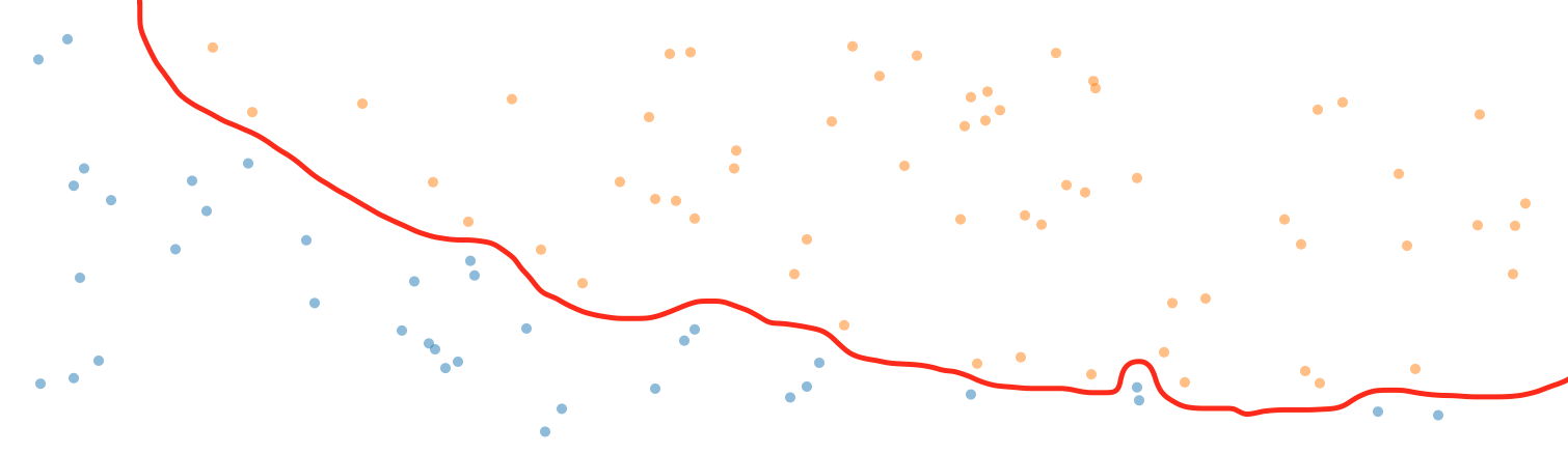
To achieve this kind of decision boundary would be marvelous, right? Well; actually it wouldn’t. Decision boundaries like this are a prototypical example of overfitting. Overfitting means that our model has adjusted itself too much to our data, and is therefore unlikely to perform well when asked to classify samples it has never seen before. Instead, what we want is a decision boundary that follows the principle of Occam’s Razor: It needs to define the boundary according to the simplest overall trends in the data by disregarding the fluctuations of random noise.

So, however counterintuitive it may seem at first, we don’t want overfitting. However, a simple linear (or slightly curved) decision boundary would also inevitably entail some level of uncertainty about our classification. Wouldn’t it be better if we could estimate the probability of an applicant being admitted rather than a black and white binary prediction?

This is what separates regression from classification. When we do classification, we predict that some sample $x^{(i)}$ belongs to some class $y^{(i)}$. Regression, on the other hand, deals with estimating some real number value related to $x^{(i)}$. One example of regression would be if we tried to estimate tomorrow’s value of the S&P 500. Similarly, trying to estimate the probability that an applicant will be admitted to a university is also a regression problem.

The sigmoid function

The logistic function — in machine learning circles better known as the “sigmoid” function — is a simple mathematical function that takes an S-like shape when you plot it on a graph:

The function itself — which we will denote as $\sigma$ — can be expressed mathematically as:

€€ \sigma(z) = \frac{1}{1 + \exp(-z)} €€

Can you see from the equation why the function looks the way it does?

Besides its pretty shape, there is one thing in particular to note about the sigmoid function: No matter how big or small the value of $z$ becomes, the function always outputs a real number between 0 and 1. This is handy, since it enables us to think of $\sigma$ as outputting a probability, where $\sigma = 0.5$ when $z = 0$, and $\sigma = 1$ as $z\rightarrow\infty$. The output of $\sigma$ will thus be our estimate of the probability that an applicant will be admitted to the university.

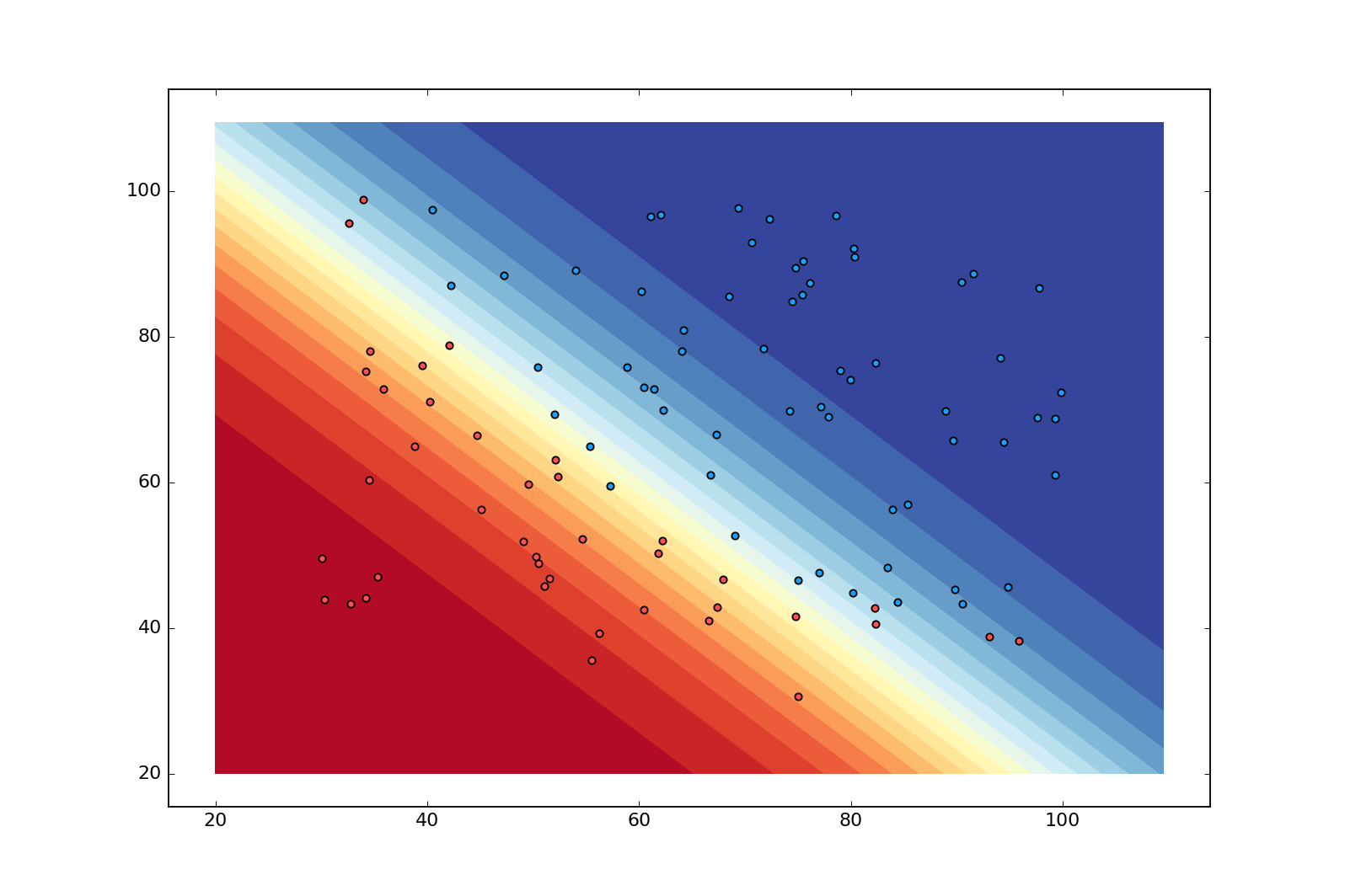
This is a contour plot showing the “decision boundary” of a model that has been trained on our dataset with logistic regression. Even though the boundary is still linear, it has now become more nuanced with the dark blue region indicating near certainty that $x^{(i)}$ is admitted ($\hat{y}^{(i)}\approx1$), and the dark red region indicating the opposite ($\hat{y}^{(i)}\approx0$). This is pretty nice since it reveals when our model is faced with uncertainty.

Defining our model

In Pt. 1, we saw how the perceptron model was a linear function of the form

€€ \theta_1x_1 + \theta_2x_2 \cdots +\theta_nx_n + b €€

where $\theta$ was an $n$-dimensional vector of weights, and $x$ was an $n$-dimensional vector of features. We also saw how we could simplify this expression by adding $b$ as an element $\theta_0$ to the vector $\theta$, and by ensuring that its corresponding element in the vector $x$ was always 1:

€€ \theta \cdot x = \begin{Bmatrix}\theta_0 \cr \theta_1 \cr \theta_2 \cr \vdots \cr \theta_n\end{Bmatrix} \cdot \begin{Bmatrix}1 \cr x_1 \cr x_2\cr \vdots \cr x_n \end{Bmatrix}= \theta_0 + \theta_1x_1 + \cdots + \theta_nx_n €€

In logistic regression, we do exactly the same. However, instead of stopping here, we feed the result of the dot product between $\theta$ and $x$ to the sigmoid function $\sigma$. Concretely, this means that given a vector $x$ containing an applicant’s exam-scores, the probability that they will be admitted to the university is calculated as:

€€ \sigma(\theta \cdot x) = \frac{1}{1+\exp(-(\theta \cdot x))} €€

The fact that we run the input data through the same linear function as the perceptron algorithm is the reason why the decision boundary remains linear. The nuance of the contour plot above is simply the result of passing the output of our linear function as a parameter to $\sigma$.

When we first initialize our logistic regression model, our parameters $\theta$ will again have random values between 0 and 1. As a result, the probabilities outputted by $\sigma$ will be way off the intended values in the beginning. To improve our parameters, we need a learning algorithm.

Quantifying errors using loss functions

The learning algorithm for logistic regression is slightly more advanced than what we saw with the perceptron in the previous post. To understand how it works, we need to familiarize ourselves with the idea of a loss function.

A loss function is a mathematical function that calculates the deviation of a prediction from the target value. Let’s see what this means by looking at the loss function for logistic regression:

€€ \frac{1}{m}\sum\limits_{i=1}^{m}-y^{(i)} \log(\hat{y}^{(i)}) - (1-y^{(i)}) \log(1-\hat{y}^{(i)}) €€

$(i)$ is the index of sample $i$, $y^{(i)}$ is the corresponding target value, and $\hat{y}^{(i)}$ is our probability estimate. $m$ is the total number of samples. Multiplying by $\frac{1}{m}$ gives us the mean loss.

Suppose we take a sample $x^{(i)}$ from our dataset with a target value $y^{(i)}$ of 1 (Admitted). When we begin training our model, it estimates the probability of $x^{(i)}$ being admitted at, say, 0.36 (a pretty bad estimate). Plugging these values into the loss function, we get:

€€ -1 \cdot \log(0.36) - 0 \cdot \log(1-0.36) €€

I have omitted the fraction and the summation, since we are only looking at the error of a single sample.

Because $y^{(i)}=1$, the second term in the expression falls away, and all we are left with is:

€€ -1 \cdot \log(0.36) \approx 0.44 €€

Now suppose we take another sample from our set; this time with a target value of 0. For simplicity’s sake, let’s assume that our probability estimate for this sample is 0.36 as well.

€€ 0 \cdot \log(0.36) - 1 \cdot \log(1-0.36) €€

This time, the first term falls away, leaving us with:

€€ -1 \cdot \log(1-0.36) \approx 0.19 €€

Notice how the loss was higher when $y^{(i)}=1$. This is exactly what we want, since our estimate of 0.36 is farther from 1 than from 0.

We know for a fact that each of our samples $x^{(i)}$ has a target value $y^{(i)}$ of either 0 or 1. It is never in between. This is nice, because it tells us that the loss for each sample can only be expressed as either $-1 \cdot \log(\hat{y}^{(i)})$ or $-1 \cdot \log(1-\hat{y}^{(i)})$. Let’s plot the two functions:

$-1 \cdot \log(\hat{y}^{(i)})$

$-1 \cdot \log(1-\hat{y}^{(i)})$

Two very useful features are evident from these plots:

1. Both functions are continuous and therefore differentiable.
2. The functions are 0 when the estimated probability $\hat{y}^{(i)}$ is equal to the target value $y^{(i)}$, and they both approach infinity as $\hat{y}^{(i)}$ moves in the opposite direction.

To see why this is useful, we need to talk about a beautiful and extremely powerful idea known as gradient descent.

Minimizing error with gradient descent

We just saw how we could quantify the error of our model’s probability estimates by using a loss function. The beauty of a loss function is that it can be effectively minimized with the help of some relatively straightforward calculus. (If your calculus is shaky, I suggest you take a crash course with Sal until you are comfortable with derivates — it is really not that bad.)

Recall that we calculate the probability of a sample $x^{(i)}$ being admitted as:

€€ \sigma(\theta \cdot x^{(i)}) = \frac{1}{1+\exp(-\theta \cdot x^{(i)})} €€

This means that $\sigma(\theta \cdot x^{(i)})=\hat{y}^{(i)}$. For clarity, let’s try to represent our complicated-looking-but-really-very-simple loss function by referring to our probability estimate this way.

€€ \frac{1}{m}\sum\limits_{i=1}^{m}-y^{(i)} \log(\hat{y}^{(i)}) - (1-y^{(i)}) \log(1-\hat{y}^{(i)}) €€ €€ \downarrow €€ €€ \frac{1}{m}\sum\limits_{i=1}^{m}-y^{(i)} \log(\sigma(\theta \cdot x^{(i)})) - (1-y^{(i)}) \log(1-\sigma(\theta \cdot x^{(i)})) €€

In the previous section, I mentioned that the loss function above is differentiable. I did not mention that the sigmoid function is as well. This is significant because — and this is where it gets cool — by having all the layers of our algorithm be differentiable, we can calculate the derivates of the loss function with respect to our parameters $\theta$! Let that sink in for a while.

What this means is that we can measure exactly how a change in our parameters $\theta$ affects a change in our loss function. When you think about it, this is unbelievably cool. In theory, you could filter $x^{(i)}$ through thousands of layers of manipulations, and as long as they are all differentiable, you can calculate how each individual one of them is affecting the final loss (and thus how to change them in order to improve your model). In fact, this is exactly how any neural network improves itself when exposed to new data. We will explore this technique in more detail in Pt 4.

The partial derivative of our loss function (which I will henceforth refer to as $C$) w.r.t. a single parameter $\theta_j$ looks like this:

€€ \frac{\partial C}{\partial \theta_j}=(\sigma(\theta \cdot x^{(i)})-y^{(i)})x_j^{(i)} €€

$j$ refers to the $j$th feature of sample $i$. If you are curious about the steps behind the derivation, check out the top-rated answer here.

A better way of writing this is to use the gradient expression:

€€ \nabla_\theta C = (\sigma(\theta \cdot x^{(i)})-y^{(i)})x^{(i)} €€

Note that $(\sigma(\theta \cdot x^{(i)})-y^{(i)})$ is a scalar, while $x^{(i)}$ is a vector.

A gradient (denoted by the symbol $\nabla$) is no more than a collection of partial derivatives. In this particular example, we have three parameters: the bias $\theta_0$ and the weights $\theta_1$ and $\theta_2$. Since we have three parameters and want to know how each one of them influences the loss $C$, we end up with three different derivatives. The gradient will therefore be a three-dimensional vector containing the derivatives for our three parameters.

You probably remember from high school that a positive derivative means that we are moving “uphill” while a negative derivative means that we are moving “downhill”. Thus, if we get a positive derivative for one of our parameters, we want the value of that particular parameter to move in the opposite direction (since moving uphill is equivalent to increasing our loss).

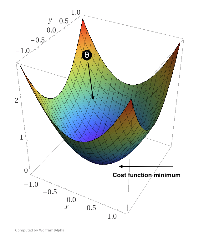
A contrived example showing how we want $\theta$ to move in the direction that minimizes the loss. Here, $\theta$ would be a two-dimensional vector.

But hold on. The above definition of our gradient only deals with a single sample! We could choose to “walk downhill” with the help of this gradient alone, but by doing that, we would only be walking down the loss function for this particular sample. To get a gradient that will improve our parameters with respect to all $n$ samples, we have to find the mean gradient like so:

€€ \nabla_\theta C = \frac{1}{m}\sum\limits_{i=1}^{m}(\sigma(\theta \cdot x^{(i)})-y^{(i)})x^{(i)} €€

That is more like it. When we perform this calculation, we get a gradient containing the mean — or distillation if you will — of all of the partial derivatives w.r.t. $\theta$ in our training set. One way to think of this is that each derivative gets to vote on which way is downhill. When we use the mean of all the votes, we move in the direction that causes a drop in the loss for the majority of our samples.

As mentioned, if the derivative for a particular parameter $\theta_j$ is positive, we want to decrease the value of $\theta_j$. Likewise, if $\theta_j$ has a negative derivative, we want to increase the value of $\theta_j$. For now, the increments by which we change $\theta_j$’s current value will simply be the same as the value of the derivatives. The following update rule describes exactly this procedure.

€€ \theta := \theta -\nabla_\theta C €€

Because of the minus sign, negative derivatives will cause the value of $\theta_j$ to increase, and positive values will cause $\theta_j$ to decrease. Exactly what we want! If we do this for enough iterations (aka. epochs), our algorithm should converge on the parameters that cause the total loss to be as small as possible. Let’s see if this works by applying what we have learned in code.

Creating a logistic regression model in Python

To create our logistic regression model, we will again be using NumPy to handle all of our matrix and vector operations as well as matplotlib to visualize what is going on. Both of these can be installed by running pip3 install numpy and pip3 install matplotlib (or simply pip if you prefer to use Python 2) on the command line. Besides NumPy and matplotlib, make sure that you also download the dataset here. Place the dataset in a dedicated folder for the project, and create a new Python file called logistic_regression.py in the same folder.

First, we will set up a LogisticRegression class. The init method will initialize an array self.theta containing our three random parameters.

import numpy as np
import matplotlib.pyplot as plt

class LogisticRegression(object):
    def __init__(self):
        super(LogisticRegression, self).__init__()
        self.theta = np.random.rand(3)

    def fit(self, X, y, epochs):
        X = self.standardize(X)
        weighted_input = np.dot(X, self.theta)
        probs = self.sigmoid(weighted_input)

        for i in range(epochs):
            gradients = self.loss_prime(probs, X, y)
            self.theta -= gradients
            weighted_input = np.dot(X, self.theta)
            probs = self.sigmoid(weighted_input)

        print("Training finished")

    def standardize(self, X):
        X_std = np.ones(np.shape(X))
        for i in range(1, X.shape[1]): # no need to standardize the x_0 column
            X_std[:, i] = (X[:, i] - np.mean(X[:, i])) / np.std(X[:, i])
        return X_std

We haven’t yet implemented all of the referenced methods, but if you analyze fit, you will see that — except for the standardize part — we have covered the theory behind everything that is happening. So, before we proceed, what does standardize do?

Standardization is done using the following formula, and forces the features of a dataset to follow a normal distribution with mean $\mu=0$ and standard deviation $\sigma=1$ (not to be confused with the sigmoid function, which we also denoted as $\sigma$).

€€ \frac{x_j^{(i)}-\mu}{\sigma} €€

Performing this trick on our particular dataset squishes the features of our first sample from around 34.62 and 78.02 down to about -1.60 and 0.63 respectively. We need to do this, because the dot product $\theta \cdot x^{(i)}$ has to be pretty small in order to avoid saturation. Saturation happens when we plug large values into the sigmoid function. This returns a number extremely close to 1, and we thus run the risk of numerical overflow and vanishing gradients. To avoid this, we use standardization to scale our features down to have zero-mean while still maintaining the ratios between the features.

We will now add the partial derivative of the loss function with respect to our parameters:

def loss_prime(self, probs, X, y):
    gradients = np.empty(np.size(self.theta))
    for i in range(len(self.theta)):
        gradients[i] = (1.0 / len(probs)) * np.sum((probs - y) * X[:, i])
    return gradients

This method outputs our gradient; an array with the same dimensions as self.theta containing one derivative per parameter. If you inspect the calculation, you will see that it is exactly the same as the gradient formula we talked about a few moments ago.

At this point, every piece of the puzzle is in place for the algorithm to train a working model. To see the fruits of our labor, though, we need to implement one last method:

def estimate(self, X):
    X = self.standardize(X)
    return self.sigmoid(np.dot(X, self.theta))

estimate will simply take a matrix (or 2D array in NumPy-speak) of samples, and return the model’s estimated probabilities of admission for each sample. We will use this method to generate a contour plot like the one we saw earlier.

Alright! Our LogisticRegression class is done; now we need to import the dataset, train the model, and make a contour plot like the one we saw earlier.

data = np.loadtxt("exam_scores.txt", delimiter=",") # importing the data
data = np.c_[np.ones((len(data), 1)), data] # making sure that x_0=1 for all samples

X = data[:, 0:3]
y = data[:, 3]

lr = LogisticRegression()
lr.fit(X, y, 100) # 100 epochs

# Creating a set of all possible exam scores between 20 and 110 in increments
# of .5. Feeding this to our trained model will color our contour plot.
xx, yy = np.mgrid[20:110:.5, 20:110:.5]
comb = np.c_[xx.ravel(), yy.ravel()]
comb = np.c_[np.ones((len(comb), 1)), comb]
probs = lr.estimate(comb).reshape(xx.shape)

f, ax = plt.subplots(figsize=(12, 8))
contour = ax.contourf(xx, yy, probs, 20, cmap="RdYlBu", vmin=0, vmax=1)

a = X[data[:, 3] == 1] # admitted samples
na = X[data[:, 3] == 0] # non-admitted samples
ax.scatter(a[:, 1], a[:, 2], c=(28.0/255, 159.0/255, 251.0/255))
ax.scatter(na[:, 1], na[:, 2], c=(252.0/255, 81.0/255, 80.0/255))

plt.show()

If you run this, you should see a contour plot exactly like the one I showed in the beginning.

Pat yourself on the back if you have followed along this far. You are now very well suited to tackle the final problem in this series: building a neural network.