How to Build (and Understand) a Neural Network Pt. 3: The Forward Pass

By now, we have covered a whole lot of material. We have talked about decision boundaries, loss functions, and gradient descent, and we have built our own linear models using the perceptron and logistic regression algorithms. In this penultimate post of the series, we will analyze the first half of a neural network — the forward pass — and we will use linear algebra to explore a visual interpretation of what happens to our data as it flows through a neural net.

A bird’s-eye view

This diagram shows a neural network composed of an input layer (green), two hidden layers (purple), and an output layer (red).

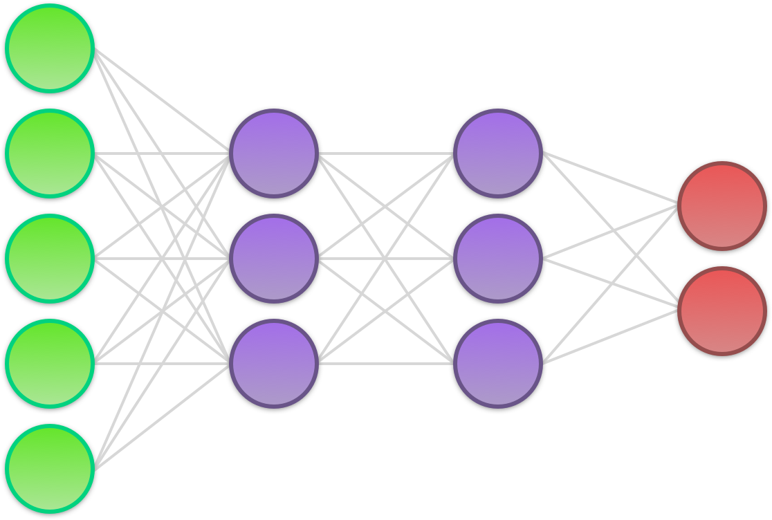
• Input layer: The input layer doesn’t do much at all; it merely represents the input of raw data to the network. The input is always a numerical representation of a piece of data (e.g. a grayscale value between 0 and 1 representing the intensity of a pixel in an image).
• Hidden layer: Above, we have two hidden layers, each consisting of three neurons. (The term ‘hidden’ is a bit silly; it refers to nothing more than the fact that the layers lie between the input and the output of the network.) The job of each hidden neuron is to apply a mathematical function to its input known as an activation function. The output of the activation function — the activation — is then passed on to the next layer in the network.
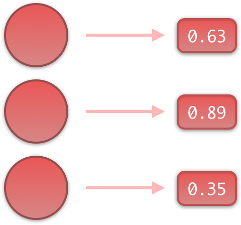
• Output layer: The output layer is the last part of a neural net. Each neuron in the output layer receives the full set of activations from the final hidden layer. On the basis of this, it then outputs a probabilistic estimate that enables us to infer something about the input data. In non-binary classification problems, there is one output neuron for each of the classes we wish to distinguish between. The output of each output neuron is the probability that a sample belongs to whatever class the output neuron represents.

Besides indicating the transfer of data, the synapses (lines) in the diagram also represent weights. As with the perceptron and logistic regression algorithms, weights are crucial to how a neural net operates. Every time a value is passed from one neuron to the next, it is multiplied by a unique weight. When we first initialize a neural net, the weights are all chosen at random. However, as we train the network, we adjust the weights up or down with the help of gradient descent to make them all converge on a combination that approximates a desired end result.

In addition to the weights, there is also a unique bias coupled to each hidden neuron and each output neuron. The biases are added to the neurons’ sum of weighted inputs before the activation function is applied.

Once a neural net has been trained, it can be used to classify unseen samples by sending them through the network and looking at the result of the output neurons. Since there are no theoretical restrictions on the number of layers and neurons, a neural network is said to be a universal function approximator, meaning that it can learn to approximate any mathematical function at all. For an in-depth exploration of this topic, see chapter four from Michael Nielsen’s free online book Neural Networks and Deep Learning.

MNIST

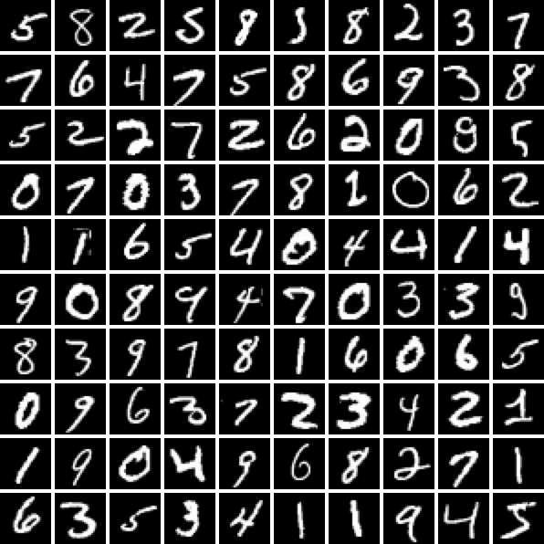
The most well-known dataset in the machine learning community (perhaps only rivalled by Iris) is called MNIST. MNIST contains 70,000 grayscale images of handwritten digits from 0-9. 60,000 of these are training samples, while the remaining 10,000 are test samples. Each image is 28x28 pixels, giving us 784 pixels per image. Because the images are all grayscale, each pixel can be represented as a floating point value between 0 and 1.

In a traditional neural network (like the one we are building today), we don’t preserve the dimensionality of the images by representing them as matrices. Instead we choose to unroll each one of them into a flat 784-dimensional vector $x$. This is in contrast to convolutional neural networks that are specifically optimized for computer vision, and need to preserve the spatial locality of every pixel.

It is intuitive to think of $x$ as a regular image with only visual qualities. However, as machine learning practitioners, we need to accustom ourselves to thinking about our data in the way that our algorithms see it; namely as a collection of numbers.

When an image is viewed as a 784-dimensional vector, we can think of it as occupying a point in 784-dimensional space. When we do this, we find that images that are visually (not conceptually) similar group together and form clusters. In the case of MNIST, this means that each digit has its own cluster in the 784-dimensional space that the images inhabit.

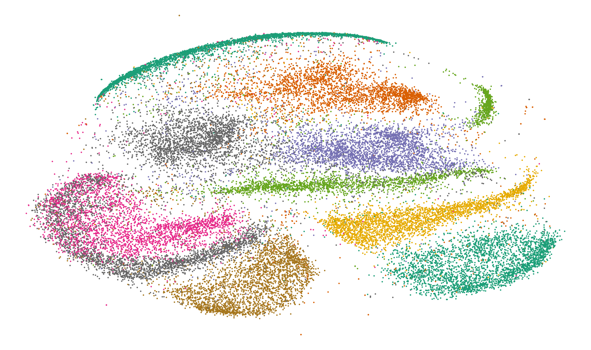
30,000 MNIST images reduced from 784 dimensions to two dimensions using t-SNE

At this point, a reasonable suggestion would be to use k-nearest neighbor to classify an image based on the cluster in which it is located. However, there is a myriad of problems with this approach: First, each digit has a fair amount of outliers (i.e. 5s that look like 6s). Second, most clusters are located very close to each other, which makes it hard to classify test samples that fall around the edges of a cluster. Additionally (and most importantly), with 60,000 training samples, it would be extremely computationally inefficient to calculate the Euclidean distance to each point before we could draw any conclusions about the data.

The million dollar question now is whether or not it is possible to minimize the amount of outliers, pull apart the clusters, and maintain computational efficiency. The answer to this question, of course, is “yes”, and we are going to demonstrate it using a neural network.

The forward pass

Before we get into the details of why neural nets work, it might be helpful to see the calculations involved in sending a mini-batch of 75 MNIST samples through a very simple, hypothetical network. This operation is called the forward pass.

Because we unroll our 28x28 images into a 784-dimensional vector, our network will have 784 input neurons. For the sake of keeping things simple, our hypothetical network will only have a single hidden layer consisting of three hidden neurons. This would not be enough for an actual neural network, but it will suffice for the purposes of this example.

Since we are looking to classify each sample as being a digit between 0-9, we will have 10 output neurons at the end of the network.

With 75 samples each containing 784 features, we can represent our mini-batch as a $784 \times 75$ matrix. Each column will thus contain the pixel values for a single image, while the rows will contain the grayscale value for the same particular pixel across our 75 different images. Since all 784 features are connected through their own “synapse” to all three hidden neurons, the weights between the input layer and the hidden layer can be represented as a $3 \times 784$ matrix.

To follow along from here, make sure that you are familiar with matrix multiplication.

Using a single matrix multiplication, we can represent the multiplication of all $784 \times 75$ features with their corresponding weight as well as each hidden neuron’s summation of its weighted input. With the columns representing samples, our input matrix $X$ looks like this:

€€ \begin{bmatrix} x_{1,1} & x_{1,2} & \cdots & x_{1,75} \cr\cr \vdots & \vdots & \vdots & \vdots \cr\cr x_{784,1} & x_{784,2} & \cdots & x_{784,75} \end{bmatrix} €€

In our first weight matrix $\Theta^{(1)}$, the rows represent the weights that lead to each particular hidden neuron. With three hidden neurons, this gives us a $3 \times 784$ matrix:

€€ \begin{bmatrix} \theta_{1,1} & \theta_{1,2} & \cdots & \theta_{1,784} \cr\cr \theta_{2,1} & \theta_{2,2} & \cdots & \theta_{2,784} \cr\cr \theta_{3,1} & \theta_{3,2} & \cdots & \theta_{3,784} \end{bmatrix} €€

When we multiply $\Theta^{(1)}$ and $X$, we get the matrix below. (Note that subscript $*$ either signifies entire rows or entire columns, such that $\theta_{i *}$ means “the entire $i$th row of $\Theta$”, and $\theta_{* j}$ means “the entire $j$th column of $\Theta$”.)

€€ \Theta^{(1)}X=\begin{bmatrix} \theta_{1 *}x_{* 1} & \theta_{1 *}x_{* 2} & \cdots & \theta_{1 *}x_{* 75} \cr\cr \theta_{2 *}x_{* 1} & \theta_{2 *}x_{* 2} & \cdots & \theta_{2 *}x_{* 75} \cr\cr \theta_{3 *}x_{* 1} & \theta_{3 *}x_{* 2} & \cdots & \theta_{3 *}x_{* 75} \end{bmatrix} €€

Our matrix of samples $X$ contains 75 column vectors $x_{* i}$, while our matrix of weights $\Theta^{(1)}$ contains 3 row vectors $\theta_{j *}$. When we multiply these, every column vector (sample) in $X$ is dotted with every row vector in $\Theta^{(1)}$. This yields a new $3 \times 75$ matrix that contains the sum of the weighted inputs for all three hidden neurons and for all 75 samples.

An easy way to remember the dynamics of matrix multiplication is that a matrix of dimensions $A \times B$ multiplied with a matrix of dimensions $B \times D$ results in a matrix of dimensions $A \times D$. Thus, when we multiply a $3 \times 784$ matrix with a $784 \times 75$ matrix, we get a $3 \times 75$ matrix.

For practical reasons that we will see later, our biases are kept in their own self-contained vector. Since each hidden neuron has its own bias, the bias vector for the hidden layer $b^{(1)}$ has dimensions $3 \times 1$. To proceed with the forward pass, we add $b^{(1)}$ to each column vector in our $3 \times 75$ matrix. This yields a new matrix $Z^{(1)}$.

Now that we have a matrix containing the sum of the weighted inputs for all three hidden neurons and for all 75 samples, we need to pass it through a nonlinear activation function (we will see why this is later). Just as in Pt. 2, we will be using the logistic sigmoid function:

€€ \sigma(z) = \frac{1}{1+\exp(-z)} €€

Once we apply the sigmoid function element-wise to the sums of the weighted inputs, we have the full set of activations from the hidden layer in the form of a matrix $A$. Like $Z^{(1)}$, $A$ has dimensions $3 \times 75$. In order to send the activations on through the network, they need to be multiplied with the second set of weights $\Theta^{(2)}$ (this is the one between the hidden layer and the output layer). Because we have three hidden neurons and 10 output neurons, the dimensions of the second weight matrix will be $10 \times 3$.

Now we can multiply our $10 \times 3$ weight matrix with the $3 \times 75$ activations. This gives us a new $10 \times 75$ matrix. Adding the 10-dimensional bias vector $b^{(2)}$ to each of the 75 column vectors yields a matrix containing the sums of the weighted inputs $Z^{(2)}$ for the output layer.

At this point, we are almost finished. Now we just need to convert the sums of the weighted inputs to the output layer $Z^{(2)}$ into the actual output of the network $\hat{Y}$. It might be tempting to apply the sigmoid function again, but doing so would end up posing a problem.

You may remember from previously that we interpreted the output of the sigmoid function as the probability of a sample belonging to one of two classes. In a neural network with multiple output neurons however, if we apply the sigmoid function at the output layer, the output of each neuron will be independent from all the others. This would produce an undesirable consequence; namely that we would be unable to interpret the output of the network as a probability distribution.

To avoid this problem, we will instead be using a function known as the softmax function, which will only be applied at the output layer.

€€ \hat{y}_{i,j} = \text{softmax}({z_{i, j}}) = \frac{\exp({z_{i,j})}}{\sum\limits_{k=1}^{n}\exp(z_{k,j})} €€

Here, $z_{i, j}$ is the summed input to output neuron $i$ for sample $j$. With 10 output neurons and 75 samples, $i$ would thus range from 1 to 10, and $j$ from 1 to 75. $n$ is the number of outputs for each sample, and is therefore equal to the number of output neurons.

Can you tell what the function does by looking at the expression?

By placing $\exp(z_{i,j})$ in the numerator and $\sum\limits_{k=1}^{n}\exp(z_{k,j})$ in the denominator, we ensure that the output of the network for each sample always sums to 1. Now, when the network outputs vectors of numbers, we can interpret the output as a probability distribution. This allows us to then choose to classify the sample as belonging to whatever class the output neuron with the highest probability represents.

This marks the end of the forward pass. Now to some intuition!

What is actually happening here?

Now that we have seen what a neural network does, it is time to answer the question of why it works. As explained by Chris Olah, the process can be separated into three distinct steps: linear transformations, translations, and applications of a nonlinearity.

Linear transformations and translations: A linear transformation scales, skews, or rotates a coordinate space by redefining the directions and amplitudes of its basis vectors. In the case of a 2D coordinate space, the only two basis vectors — $\bar{x}$ and $\bar{y}$ — are defined as $\begin{bmatrix}1 \cr 0 \end{bmatrix}$ and $\begin{bmatrix}0 \cr 1 \end{bmatrix}$ respectively. While they may not look like much, $\bar{x}$ and $\bar{y}$ fully define their own coordinate space. To see why, let us first join them into a matrix:

€€ \begin{bmatrix}1 & 0 \cr 0 & 1 \end{bmatrix} €€

Then, let us take an arbitrary point $\begin{bmatrix}x \cr y \end{bmatrix}$ and multiply it by our matrix:

€€ \begin{bmatrix}1 & 0 \cr 0 & 1 \end{bmatrix} \begin{bmatrix}x \cr y \end{bmatrix} = \begin{bmatrix}1x+0y \cr 0x+1y \end{bmatrix} = \begin{bmatrix}x \cr y \end{bmatrix} €€

Using matrix-vector multiplication, we just showed that in a coordinate space with these basis vectors, the point $\begin{bmatrix}x \cr y \end{bmatrix}$ remains unchanged.

Now let’s see what happens when we double $\bar{x}$:

€€ \begin{bmatrix}2 & 0 \cr 0 & 1 \end{bmatrix} \begin{bmatrix}x \cr y \end{bmatrix} = \begin{bmatrix}2x+0y \cr 0x+1y \end{bmatrix} = \begin{bmatrix}2x \cr y \end{bmatrix} €€

Here, the original point $\begin{bmatrix}x \cr y \end{bmatrix}$ gets moved to $\begin{bmatrix}2x \cr y \end{bmatrix}$ when we apply the transformation. Since this is true of all points, we can visualize this as a transformation of the space itself:

Pretty straightforward, right? Now, let’s do something a little more interesting. Instead of merely shrinking or stretching the axes, let’s try to make them codependent. For instance, we could define a transformation like this:

€€ \begin{bmatrix}2 & 0 \cr 1 & 1 \end{bmatrix} \begin{bmatrix}x \cr y \end{bmatrix} = \begin{bmatrix}2x+0y \cr 1x+1y \end{bmatrix} = \begin{bmatrix}2x \cr x+y \end{bmatrix} €€

This transformation — known as a shear — has the effect that every time we increase $x$ by 1, we also increase $y$ by 1. Let’s visualize this to gain some intuition:

Now it is easier to see what is happening. As soon as we begin increasing $x$, not only are we moving to the right, but also upwards. In this transformed space, it is impossible to change $x$ without also changing $y$. A change in $y$, however, does not affect $x$, since the y-axis remains orthogonal to the original x-axis.

When we pass data into a neural network, this kind of transformation is what happens during the weight multiplication. One thing to note, however, is that the number of hidden neurons in each layer might be smaller or larger than the number of neurons in the layer that preceded it. This results in the dimensionality of the data either getting reduced or expanded as it passes through the network. If there are more neurons in the first hidden layer than in the input layer, this causes the dimensionality of the data to be expanded. Likewise, if there are less hidden neurons than input neurons, the dimensionality will be reduced.

Adding a unique bias to each hidden or output neuron has the effect of translating the space; that is, pushing or pulling our data in different directions for each dimension. Again, let’s see what this looks like:

Here, we first transform the space, and then translate it by $\begin{bmatrix}3 \cr 2 \end{bmatrix}$. Note that unless we keep the original space in the background, translations can be hard to visualize while properly keeping the space in view. I will therefore ignore them in future visualizations.

Finally — and perhaps most significantly — is the effect of applying a nonlinear activation function (like the logistic sigmoid function). This takes all the points of the space and applies the function to each of the point’s components individually.

The “nonlinear” part is important here. As opposed to linear transformations like the ones we just saw, nonlinear transformations are able to warp space in very dynamic and elastic ways. As shown below, this can make for some quite beautiful visualizations.

As you can see, the shape of a space transformed by a sigmoid function is highly dependent on the space to which it is applied. This is why the weights and biases are so important; they do the groundwork that lets the activation function bend the data in the most optimal way.

But what is “the most optimal way?” To answer this question, we need to turn our eyes to the output layer. As we touched on in Pt. 1, the equation for a hyperplane can be expressed as the variables (${x_1, \cdots, x_n}$) that, when multiplied by their corresponding coefficient (${y_1, \cdots, y_n}$), sums to 0:

€€ x_1y_1 + x_2y_2 + \cdots + x_ny_n=0 €€

We also saw how the exact same thing could be expressed as the dot product between vectors:

€€ x \cdot y = 0 €€

When we have a set of activations that pass from the final hidden layer of a neural net to the output layer, we are essentially taking the vector dot product between the activations and the set of weights that lead to a particular output neuron. Each neuron then runs its input through the softmax function and interprets the output as a probability distribution over the (mutually exclusive) classes that the neurons represent.

Sounds familiar to logistic regression? That’s because it is. In fact, using the softmax function to generate probability distributions is also known as multinomial logistic regression.

This tells us something really interesting: In order for the output layer to distinguish between different classes, it needs to be able to separate them with a straight line just as in Pt. 1 and Pt. 2. However, where the perceptron and logistic regression algorithms could only handle data that was linearly separable from the get-go, a neural net takes its input data and transforms it into becoming linearly separable if it isn’t already!

This is the same dataset as the one we used in the previous post. Unlike our logistic regression algorithm however, a neural net is able to perfectly distinguish between the classes because the output layer only sees the space in which they are linearly separable.

The code

A thing that surprised me when I set up my first neural network was the brevity of the actual program. While the underlying concepts can sometimes be a challenge to fully grasp, the number of lines of code required to build one is actually very modest.

Let’s begin by setting up a NeuralNetwork class in a file called neural_network.py. We will use the __init__ method to instantiate our hyperparameters:

import numpy as np

class NeuralNetwork(object):
    def __init__(self, layer_sizes, alpha=0.1):
        super(NeuralNetwork, self).__init__()

        n_layers = len(layer_sizes)

        if (n_layers >= 3):
            self.thetas = []
            self.biases = []

            for i in range(n_layers-1): # a network with n layers has n-1 set of weights and biases
                self.thetas.append(np.random.randn(layer_sizes[i+1], layer_sizes[i]))
                self.biases.append(np.random.randn(layer_sizes[i+1], 1))

            self.thetas = np.array(self.thetas)
            self.biases = np.array(self.biases)
            self.alpha = alpha
        else:
            raise ValueError("The minimum number of layers is 3 (%i provided)" % n_layers)

Our __init__ method takes two arguments: layer_sizes and alpha. layer_sizes will be a list of numbers specifying the size (number of neurons) of each layer in the network. Therefore, it will also implicitly define the size of the network itself. There is no need to worry about the alpha argument just yet; we will explore what it means in the next post.

To implement the forward pass, we will add a forward_pass method to NeuralNetwork:

def forward_pass(self, A):
    Zs = []
    As = [A]

    for i in range(len(self.thetas)):
        Z = np.dot(self.thetas[i], As[-1]) + self.biases[i]
        Zs.append(Z)

        if i < len(self.thetas)-1:
            As.append(self.sigmoid(Z))
        else:
            Y_hat = self.softmax(Z)

    return (Zs, As, Y_hat)

def sigmoid(self, Z): return 1.0 / (1.0 + np.exp(-Z))
def softmax(self, Z): return np.exp(Z) / np.sum(np.exp(Z), axis=0)

Here, forward_pass takes the activations of the first layer A (aka. the raw input), and runs it through the network. It completes by returning the following:

• A list Zs containing matrices of weighted inputs for the hidden layers and the output layer.
• A list As containing matrices of activations for each hidden layer.
• A matrix Y_hat containing the probability distribution over all possible classes and for all samples in A.

This concludes our implementation of the forward pass for our neural network. In the next (and final) post of the series, we will explore how our network can automatically find the right values for our weights and biases using backpropagation.