Proportional Reward Sampling With GFlowNets

November 13, 2022

Code available on GitHub

Imagine a chemist in search of a novel drug that will bind to a specific protein in the human body. The chemist is faced with two problems: 1) The space of possible drugs is enormous and 2) the cost of synthesizing a large variety of candidate drugs and evaluating their efficacy is prohibitively expensive and time-consuming.

To help her automate the process of finding a small set of candidate drugs, she trains an oracle model to output a score for any arbitrary molecule indicating how well it will bind to the target protein. This is done in a supervised fashion by training the model on $(x,y)$ pairs, where $x$ represents known drugs and $y$ is the efficacy with which the drug binds to the protein. This model, however, is not generative, and will not help her find the novel compound she is looking for on its own. This is where Generative Flow Networks (GFlowNets) enter the picture.

Overview

GFlowNets were proposed in 2021 by Emmanuel and Yoshua Bengio (and collaborators) at Mila ¹ and attempt to solve two problems simultaneously: The first problem is that of sampling discrete and composite objects $x$ (i.e. any object which can be built by adding up elements in a sequence of discrete steps). For instance, graphs and molecules are examples of such objects, since they can be sampled by adding nodes/atoms and edges/bonds to the object one step at a time.

The second problem is that of sampling such objects in proportion to a given non-negative reward or “energy” function $R(x)$. The key phrase here is “in proportion to.” Usually, models are trained to maximize a given reward function, thus converging around one or a few high-reward samples. In contrast, a GFlowNet is trained such that the probability $p(x)$ of sampling an object $x \in \mathcal{X}$ matches that of the normalized reward, i.e.

€€p(x) = \frac{R(x)}{\sum_{x’ \in \mathcal{X}} R(x’)}.€€

This property encourages exploration of the sample space $\mathcal{X}$ and will tend to produce a wider variety of samples than the ones obtained from a model trained using reward maximization. While this property is not always desirable, it is likely to be very useful for our hypothetical chemist. This is because the oracle is only approximate and will thus occasionally assign lower scores than are warranted to novel compounds that are, in fact, excellent at binding to the target protein. The question, then, is how do GFlowNets achieve this?

Sampling

The novelty of GFlowNets lies in the way they are trained rather than in the details of their architecture. In fact, more or less any neural network can act as the architecture for a GFlowNet. To understand how the architecture is trained, however, we need to take a closer look at how the authors formulate the problem of sampling from the model.

Consider the problem of sampling three-node DAGs. For a three-node graph with nodes $X$, $Y$ and $Z$, there are 25 possible DAGs, many of which can be arrived at in multiple ways starting from the empty graph (i.e. the graph with three nodes but no edges). Let $s_0$ denote the empty graph and the starting point of the sampling process. From here, we have a set of allowed actions $\mathcal{A}(s_0)$ that will add an edge to the empty graph (or terminate, since $s_0$ is a valid DAG). Specifically, we can choose between the following actions:

€€ \begin{aligned} \mathcal{A}(s_0) = \lbrace &X \rightarrow Y, \newline &X \leftarrow Y, \newline &Y \rightarrow Z, \newline &Y \leftarrow Z, \newline &X \rightarrow Z, \newline &X \leftarrow Z, \newline &\text{terminate} \rbrace, \end{aligned} €€

each one transitioning to either of $s_1,…,s_6$ or terminating at $s_0$. Since there are 25 possible DAGs, the state space is $s_0,…,s_{24}$. (In general, not all states need to correspond to valid objects. When $s_i$ represents an invalid object, $\mathcal{A}(s_i)$ will simply not contain the $\text{terminate}$ action. This is useful in cases where the model needs to “pass through” an invalid object to reach a valid one.) We can visualize a small part of the state-action space in the following way:

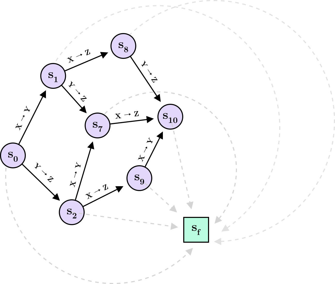
Here I have restricted the space to include only the states and actions resulting from initially choosing $X \rightarrow Y$ or $Y \rightarrow Z$ and leading to the DAG with edges $(X \rightarrow Y, Y \rightarrow Z, X \rightarrow Z)$. It is clear from the diagram that there can be multiple action sequences leading to the same state. An action sequence can also be thought of as a trajectory $\tau$, such that $\tau = (s_0 \rightarrow \cdots \rightarrow s_T \rightarrow s_f)$ contains the history of how the final object $s_T$ was constructed step-by-step. You will also notice a special state $s_f$. This state is known as the sink and is reached whenever sampling terminates. The sink is not part of the model as such but—as we will see below—is helpful in formalizing a training objective.

Flow

The main idea behind GFlowNets is to imagine $Z = \sum_{x \in \mathcal{X}} R(x)$ units of water flowing from the source $s_0$ along the various trajectories and exiting the system through the sink. Crucially, for a state $s$ representing an object $x$, the amount of flow on the path $s \rightarrow s_f$ should equal $R(x)$ while any excess flow should pass onto other states. If we can achieve this, the relative frequency of terminating at $s$ for any unit of flow will be $\frac{R(x)}{Z}$, and we will thus be sampling $x$ in proportion to its reward. The difficulty is to formalize a loss for which the optimal solution obeys this restriction. To do so, we need to introduce the flow matching conditions.

Flow matching and trajectory balance

Let $F(s \rightarrow s’)$ denote the flow along the path $s \rightarrow s’$, and let $\text{Pa}(s)$ and $\text{Ch}(s)$ denote the parent states and child states of $s$, respectively. In order for a flow to be valid, the following condition needs to hold for all states other than $s_0$ and $s_f$ ²:

€€ \sum_{s’ \in \text{Pa}(s)} F(s’ \rightarrow s) = \sum_{s’’ \in \text{Ch}(s)} F(s \rightarrow s’’) + R(s) \tag{1} €€

For convenience, we assume $s_f \notin \text{Ch}(s)$ for any $s$. This means that the equality enforces that the terminal flow $F(s \rightarrow s_f)$ must equal $R(s)$ while any excess flow is distributed among the child states in $\text{Ch}(s)$. There are multiple ways to do this. For instance, you might introduce a flow estimator $F_\phi$ with parameters $\phi$ and minimize the flow matching loss

€€ \mathcal{L}_{FM}(s) = \left( \log \frac{\sum_{s’ \in \text{Pa}(s)} F_\phi (s’ \rightarrow s)}{\sum_{s’’ \in \text{Ch}(s)} F_\phi (s \rightarrow s’’) + R(s)} \right)^2. €€

An alternative (but equivalent) approach is to formulate the problem in terms of a forward policy $P_F(s_{t+1} \mid s_t)$ outputting a distribution over states reachable from the state at time $t$ (you could also view this as a distribution over $\mathcal{A}(s_t)$) as well as an estimate $Z_\theta$ of the total flow originating from $s_0$. Further, if we introduce a backward policy $P_B(s_t \mid s_{t+1})$, we can formulate what is known as the trajectory balance loss ³:

€€ \mathcal{L}_{TB}(\tau) = \left( \log \frac{Z_\theta \prod_{t=1}^T P_F(s_{t+1} \mid s_t)}{R(s_T) \prod_{t=1}^T P_B(s_t \mid s_{t+1})} \right) ^2 : \tau = (s_0 \rightarrow \cdots \rightarrow s_T \rightarrow s_f) €€

To understand the trajectory balance loss, consider the detailed balance condition, which simply states that $F(s \rightarrow s’)$ can be expressed both as a fraction of the total flow $F(s)$ through $s$ and as a fraction of the total flow $F(s’)$ through $s’$:

€€ P_F(s’ \mid s)F(s) = P_B(s \mid s’)F(s’) \tag{2} €€

If this is not intuitive, imagine that Alice and Bob each have 10 liters of water. Alice hands 8 liters to Charlie while Bob hands him 5 liters. The water “flowing between” Alice and Charlie is $0.8 \cdot 10$ but can also be expressed as $\frac{8}{13} \cdot 13$, since Charlie receives 13 liters in total. When $P_F$ and $P_B$ agree in this way, they satisfy the detailed balance condition.

Inspired by this, the trajectory balance loss replaces the flow $F(s’)$ on the right-hand side in (2) with the reward $R(s’)$. Note that this is only done with respect to the last state of a trajectory (i.e. $s_f$), since this is the only state to which the flow from $s_T$ should always exactly equal the reward $R(s_T)$. Interestingly, the authors argue that there is a unique flow satisfying the flow matching condition in (1) regardless of the choice of $P_B$. We can thus safely set $P_B$ to a uniform distribution over the parent states and focus our attention solely on training $Z_\theta$ and $P_F$.

Implementing a GFlowNet

We will now follow in the footsteps of Bengio et al. ² and implement a GFlowNet to model a two-dimensional grid environment in which each coordinate has a corresponding reward. $s_0$ will represent the upper-left-hand coordinate, and each action will move down or right of the current coordinate. For a grid size of $N=16$, the reward “environment” looks like this:

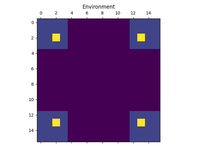
As can be seen from the image, the reward function has four modes separated by “dead zones” with very low reward. The lower the reward, the harder it will be for the model to explore the environment. In the extreme case of the reward being 0 outside of the modes, the model will be unable to explore the environment, as no flow will be able to pass through the dead zones. As long as the reward is positive, however, the model will be able to explore the entire environment given enough time.

We are going to implement $P_F$ as a small MLP taking as input an $N^2$-dimensional one-hot vector indicating the current position (state), and outputting a distribution over possible actions: $\text{Down}$, $\text{Right}$ or $\text{Terminate}$. When the current position is at the bottom or right edge of the environment, the invalid action of $\text{Down}$ or $\text{Right}$ will be masked by setting its probability to 0. Finally, we sample an action according to this distribution, update the state accordingly, input the new state to $P_F$, etc. This goes on until the model chooses the $\text{Terminate}$ action after which we compute the trajectory balance loss and update $Z_\theta$ and $P_F$. Rinse and repeat.

Let’s start with implementing the forward and backward policy.

class ForwardPolicy(nn.Module):
    def __init__(self, state_dim, hidden_dim, num_actions):
        super().__init__()
        self.dense1 = nn.Linear(state_dim, hidden_dim)
        self.dense2 = nn.Linear(hidden_dim, num_actions)
    
    def forward(self, s):
        x = self.dense1(s)
        x = relu(x)
        x = self.dense2(x)
        return softmax(x, dim=1)
        
class BackwardPolicy:
    def __init__(self, state_dim, num_actions):
        super().__init__()
        self.num_actions = num_actions
        self.size = int(state_dim**0.5)
    
    def __call__(self, s):
        idx = s.argmax(-1)
        at_top_edge = idx < self.size
        at_left_edge = (idx > 0) & (idx % self.size == 0)
        
        probs = 0.5 * torch.ones(len(s), self.num_actions)
        probs[at_left_edge] = torch.Tensor([1, 0, 0]) # previous action was "down"
        probs[at_top_edge] = torch.Tensor([0, 1, 0]) # previous action was "right"
        probs[:, -1] = 0 # disregard termination action
        
        return probs

The most interesting part here is BackwardPolicy. Since we use a fixed backward policy, the class does not need to inherit from nn.Module. When given a state, the __call__ method simply defaults to assigning $0.5$ probability to having arrived at the state from either of the two parent states (top or left). However, in the case where there is only one parent state (at the left and top edge of the environment), we set the probability to $1$ for the single parent state.

We also define a Grid class responsible for masking invalid actions, taking state-action pairs and outputting updated states, and computing state rewards.

class Grid:
    def __init__(self, size):
        self.size = size
        self.state_dim = size**2
        self.num_actions = 3 # down, right, terminate
        
    def update(self, s, actions):
        idx = s.argmax(1)
        down, right = actions == 0, actions == 1
        idx[down] = idx[down] + self.size
        idx[right] = idx[right] + 1
        return one_hot(idx, self.state_dim).float()
    
    def mask(self, s):
        mask = torch.ones(len(s), self.num_actions)
        idx = s.argmax(1) + 1
        at_right_edge = (idx > 0) & (idx % (self.size) == 0)
        at_bottom_edge = idx > self.size*(self.size-1)
        mask[at_right_edge, 1] = 0
        mask[at_bottom_edge, 0] = 0
        return mask
        
    def reward(self, s):
        grid = s.view(len(s), self.size, self.size)
        coord = (grid == 1).nonzero()[:, 1:].view(len(s), 2)
        R0, R1, R2 = 1e-2, 0.5, 2
        norm = torch.abs(coord / (self.size-1) - 0.5)
        R1_term = torch.prod(0.25 < norm, dim=1)
        R2_term = torch.prod((0.3 < norm) & (norm < 0.4), dim=1)
        return (R0 + R1*R1_term + R2*R2_term)

Finally, we implement the actual GFlowNet.

class GFlowNet(nn.Module):
    def __init__(self, forward_policy, backward_policy, env):
        super().__init__()
        self.total_flow = Parameter(torch.ones(1))
        self.forward_policy = forward_policy
        self.backward_policy = backward_policy
        self.env = env
    
    def mask_and_normalize(self, s, probs):
        probs = self.env.mask(s) * probs
        return probs / probs.sum(1).unsqueeze(1)
    
    def forward_probs(self, s):
        probs = self.forward_policy(s)
        return self.mask_and_normalize(s, probs)
    
    def sample_states(self, s0, return_log=False):
        s = s0.clone()
        done = torch.BoolTensor([False] * len(s))
        log = Log(s0, self.backward_policy, self.total_flow, self.env) if return_log else None

        while not done.all():
            probs = self.forward_probs(s[~done])
            actions = Categorical(probs).sample()
            s[~done] = self.env.update(s[~done], actions)
            
            if return_log:
                log.log(s, probs, actions, done)
                
            terminated = actions == probs.shape[-1] - 1
            done[~done] = terminated
        
        return (s, log) if return_log else s

The sample_states method takes as input the initial states s0 and loops until all states have terminated. The Log class is responsible for logging the current estimate of the total flow, the reward for each sample, and the forward and backward probabilities encountered along the trajectory for each sample. These are logged, since they are required to compute the trajectory balance loss. I won’t go into detail with the implementation of Log here but feel free to check it out on GitHub.

We are now ready to train the GFlowNet.

def train(batch_size, num_epochs):
    env = Grid(size=size)
    forward_policy = ForwardPolicy(env.state_dim, hidden_dim=32, num_actions=env.num_actions)
    backward_policy = BackwardPolicy(env.state_dim, num_actions=env.num_actions)
    model = GFlowNet(forward_policy, backward_policy, env)
    opt = Adam(model.parameters(), lr=5e-3)
    
    for i in (p := tqdm(range(num_epochs))):
        s0 = one_hot(torch.zeros(batch_size).long(), env.state_dim).float()
        s, log = model.sample_states(s0, return_log=True)
        loss = trajectory_balance_loss(log.total_flow,
                                       log.rewards,
                                       log.fwd_probs,
                                       log.back_probs)
        loss.backward()
        opt.step()
        opt.zero_grad()
        if i % 10 == 0: p.set_description(f"{loss.item():.3f}")

Once the model has been trained, we can sample a final batch of $10,000$ samples from the sample_states method, this time without needing the logged data.

s0 = one_hot(torch.zeros(10**4).long(), env.state_dim).float()
s = model.sample_states(s0, return_log=False)
plot(s, env)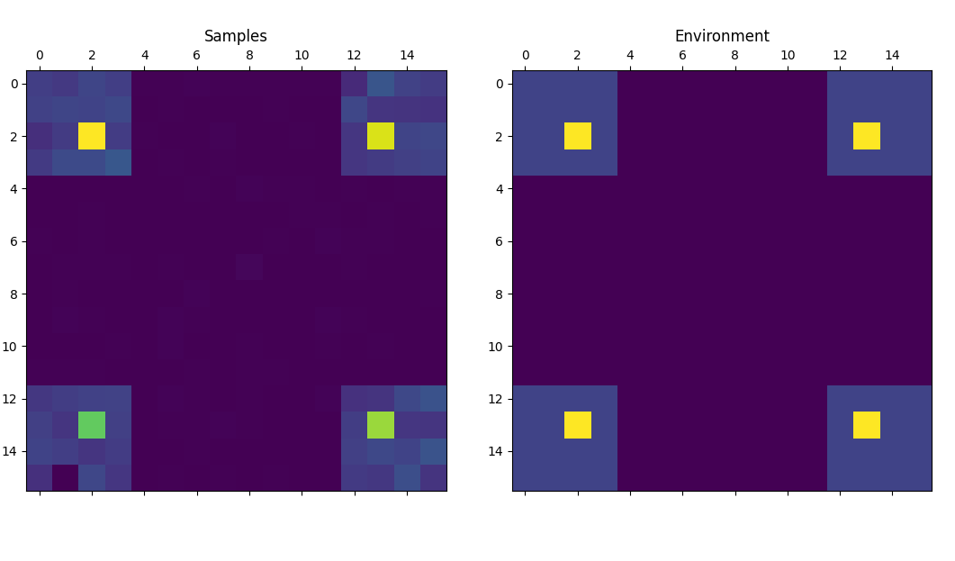

As you can see, the relative frequency of each sample from the trained model (left) is roughly proportionate to its corresponding reward (right). Of course, this is a simple toy problem that serves only as a proof of concept. For an example on how GFlowNets can be applied to more real-world problems, see for instance the recent work of Deleu et al. ⁴ on using GFlowNets for Bayesian structure learning.

Conclusion

GFlowNets are a new area of research and time will tell how useful they will turn out to be. To me, they seem like a promising tool for problems such as drug discovery and causal inference, where the objects of interest are discrete (i.e. molecules and causal graphs) and where the prediction of oracle models or the evaluation of likelihoods can serve as reward functions. If you are interested in more of the thoughts behind GFlowNets, I highly recommend the MLST interview with Yoshua Bengio.

References