Transformer-XL: A Memory-Augmented Transformer

December 3, 2022

Code available on GitHub

In this post, we will implement a lightweight version of the Transformer-XL model. Proposed by Dai et al. in 2019¹, Transformer-XL introduced two innovations that, when combined, enable the attention mechanism to have a wider “field of view” and result in significant performance improvements on autoregressive evaluation. A variant of Transformer-XL constitutes the backbone of XLNet², a highly popular pretrained language model proposed in 2020 by the same authors.

Inspired by minGPT, our implementation of Transformer-XL will be trained for the somewhat mundane task of sorting unordered sequences of numbers. Simple tasks like these minimize boilerplate code, allow us to focus on conceptual clarity, and don’t require access to fast GPUs.

Context fragmentation

In a “vanilla” Transformer architecture trained for tasks such as language modeling or sentiment analysis, the model takes as input fixed-length segments of $L$ words (or, more specifically, tokens). Using the self-attention mechanism then allows the model to discover relationships between words in the segment that are relevant for the task at hand.

However, as the name implies, self-attention is restricted to looking at the segment itself, and it is thus unable to pick up on long-range ($>L$) dependencies between words. This problem is exacerbated by the fact that segments are constructed by selecting consecutive $L$-size chunks of text with no consideration for semantic boundaries. This can be problematic for language modeling, where predicting the words of segment $k$ often requires knowledge of the words in segment $k-1$. Dai et al. refer to this problem as context fragmentation.

Recurrent memory

To address the problem of context fragmentation, the authors of Transformer-XL propose to augment the original Transformer architecture with a recurrent hidden state that serves to store the salient features of previous segments. Concretely, let $\textbf{s}_{k-1} = [x^{(1)}_{k-1},…, x^{(L)}_{k-1}]$ and $\textbf{s}_k = [x^{(1)}_k,…,x^{(L)}_k]$ be two consecutive length-$L$ segments. Referring to the hidden states produced by layer $n$ for segment $\textbf{s}_k$ by $H^n_k \in \R^{L \times d}$, the hidden states are produced as follows:

€€ \begin{aligned} \tilde{H}^{n-1}_{k} &= [\text{SG}(H^{n-1}_{k-1}) \mid\mid H^{n-1}_k] \newline Q, K, V &= H^{n-1}_kW_Q, \tilde{H}^{n-1}_{k} W_K, \tilde{H}^{n-1}_{k} W_V \newline H^n_k &= \text{Transformer-Layer}(Q, K, V) \end{aligned} \tag{1} €€

Here, $\mid\mid$ denotes row-wise matrix concatenation while $\text{SG}$ is the stop-gradient operator indicating that the model does not backpropagate through time. Recurrent neural networks like LSTMs³ were notoriously difficult to train for exactly this reason and it is thus avoided here.

Notice that we can already infer from the query-key-value computation that the model does not use pure self-attention. Rather, it uses a mixture of self-attention on the vectors in $H^{n-1}_k$ and cross-attention between $H^{n-1}_k$ and the hidden states $H^{n-1}_{k-1}$ produced by the previous segment. This allows the model to not only attend to words in the current segment but also to incorporate information from previous ones.

Further, since each $H^n_k$ is recurrent, a single hidden state can, in principle, contain information extending beyond the previous segment. Still, we can achieve more fine-grained control of the model’s “memory capacity” by caching any number $M$ of previous hidden states. Since $M$ can be smaller or larger than the length of a segment, we replace $H^n_{k-1} \in \R^{L \times d}$ by $H^n \in \R^{M \times d}$.

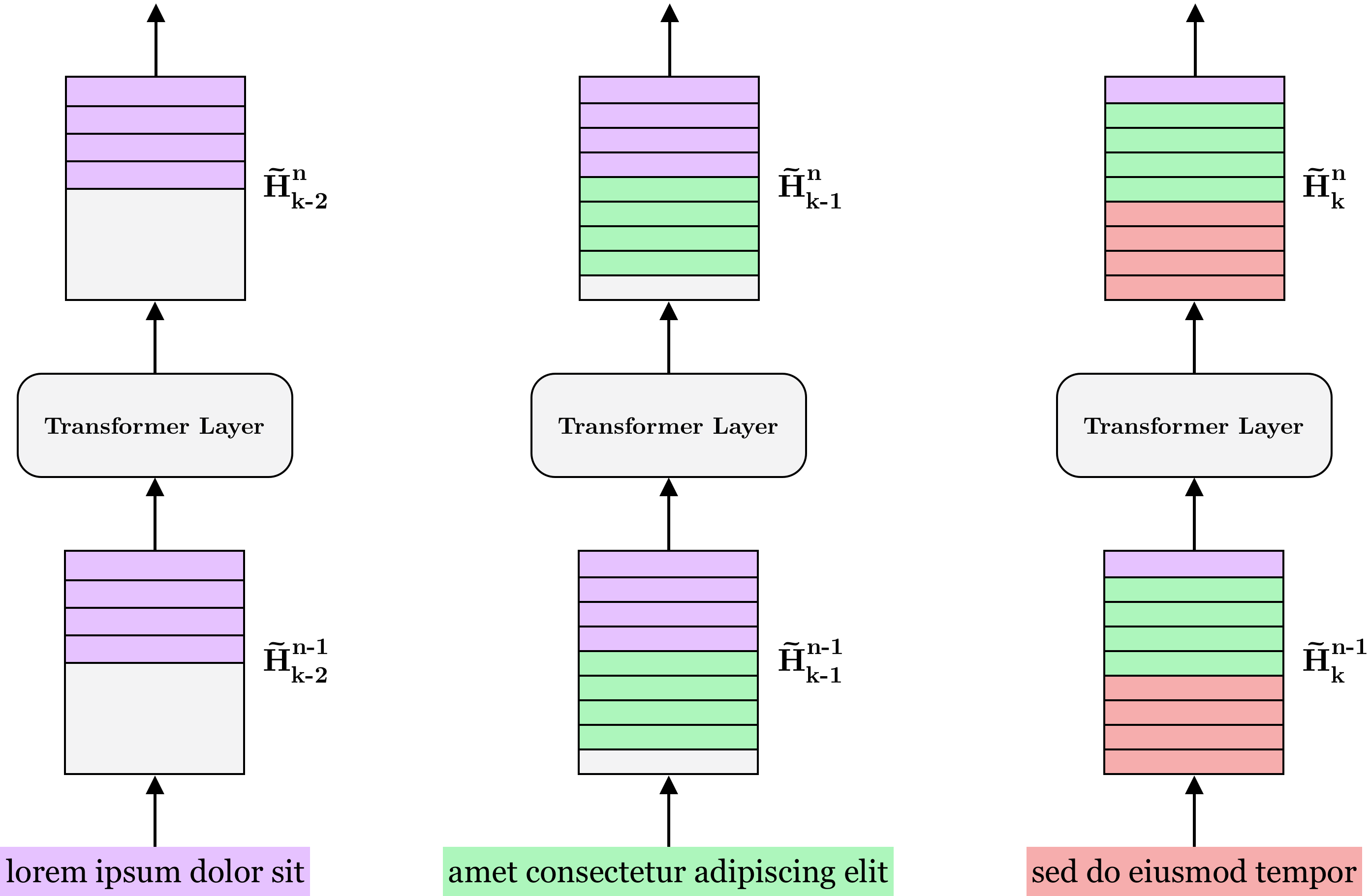
Figure 1: $M$ previous hidden states are saved to memory for each layer and input along with the representation of the current segment. Here shown with segment length $L=4$ and memory length $M=5$.

Augmenting the architecture in this way also enables significant speedups when evaluating the model autoregressively. To see why, note that it is possible to feed only the most recently generated token back into the model, since the hidden state of previous words have already been computed and saved to memory. According to the authors, this makes Transformer-XL up to 1800+ times faster on some tasks than a vanilla Transformer.

Positional encodings

One of the primary characteristics of Transformers is permutation equivariance. This means that the order in which tokens are input to the model has no effect on the output (aside from the order). For instance, if inputting $(x,y,z)$ to a Transformer outputs $(\hat{x}, \hat{y}, \hat{z})$, then inputting $(z, y, x)$ will output $(\hat{z}, \hat{y}, \hat{x})$. In practical terms, this means that the location of a word in a segment has no bearing on the model’s representation of that word.

To resolve this, Vaswani et al. introduced positional encodings⁴. A positional encoding for a word at position $l$ in a segment and with embedding $x^{(l)} \in \R^d$ is a vector $p^{(l)} \in \R^d$ in which the entries $p^{(l)}_1,…,p^{(l)}_d$ alternate between being functions of sine and cosine wave functions:

€€ p^{(l)}_i = \begin{cases} \sin(\frac{l}{1000^{2k/d}}) & \text{if } i = 2k \newline \cos(\frac{l}{1000^{2k/d}}) & \text{if } i = 2k+1 \end{cases} €€

The details of why such vectors can be used to represent positions is outside the scope of this post. However, the important thing to note is that the final embeddings input to a Transformer is simply the vector addition $x^{(l)} + p^{(l)}$. This essentially acts as a “label” to let the model know where in the segment each word is placed.

While this works extremely well in the original Transformer, it unfortunately poses a problem for the use of the hidden state memory outlined in the previous section. To see why, consider that the $l$’th word of segments $\textbf{s}_{k-1}$ and $\textbf{s}_k$ share the same positional encoding. This means that the hidden states representing information of previous segments are functions of positional encodings that continually reset, i.e. $1,…,L,1,…,L,1…,L$. This makes it harder for the model to determine how words in the current segment relate to words in previous segments and thus presents an obstacle for the use of the hidden states.

Relative positional encodings

To resolve this problem, Dai et al. propose to use relative positional encodings. These are identical to the sinusoid encodings proposed by Vaswani et al. but instead of letting $p^{(l)}$ represent the $l$’th position in a segment, it represents a distance of $l$ between two words.

To see how we might employ such encodings, recall that the pre-softmax attention score (omitting the $\frac{1}{\sqrt{d}}$ scaling factor) is $QK^\text{T}$. Remembering the query-key-value computation in $(1)$ and assuming regular positional encodings $P_Q \in \R^{L \times d}$ and $P_K \in \R^{M+L \times d}$ for the query and key vectors, respectively, we can write the attention score as

€€ (H W_Q + P_QW_Q)(\tilde{H} W_K + P_KW_K)^\text{T}, €€

where have dropped the superscript $n$ and subscript $k$ for notational clarity. We can then further decompose the above expression as follows:

€€ \underbrace{HW_Q W_K^\text{T}\tilde{H}^\text{T}}_{(a)} + \underbrace{HW_Q W_K^\text{T}P^\text{T}_K}_{(b)} + \underbrace{P_QW_Q W_K^\text{T}\tilde{H}^\text{T}}_{(c)} + \underbrace{P_QW_Q W_K^\text{T}P^\text{T}_K}_{(d)}. €€

The authors now propose the following change to the above expression, with $R$ being a matrix of relative positional encodings. (Note that this is not the notation used by Dai et al. but it captures the same idea.)

€€ \textcolor{lightgray}{\underbrace{HW_Q W_K^\text{T}\tilde{H}^\text{T}}_{(a)} +} \underbrace{\text{shift}(HW_Q W_R^\text{T}R^\text{T})}_{(b)} + \underbrace{UW_K^\text{T}\tilde{H}^\text{T}}_{(c)} + \underbrace{\text{shift}(TW_R^\text{T}R^\text{T})}_{(d)}. \tag{2} €€

First, notice that the transformed positional encodings $P_QW_Q$ for the query vectors have been replaced in $(c)$ and $(d)$ by $U$ and $T$. Both $U$ and $T$ are matrices in $\R^{L \times d}$ but have repeated rows (i.e. the rows are made up of parameters $u,t \in \R^d$ and are thus the same for every query vector⁵). This creates two complimentary effects on the attention mechanism: $(c)$ creates a global content bias that emphasizes certain words regardless of their location, while $(d)$ does the opposite by expressing a global positional bias that emphasizes certain locations regardless of the associated content.

Removing $P_QW_Q$ is the first step toward disregarding absolute positions. To see how the relative positional encodings work, first recall that the key vectors contain both the $L$ words of the current segment as well as the $M$ previous words. The matrix $R \in \R^{M+L \times d}$ contains sinusoid positional encodings with the order “flipped” such that the first row represents the biggest distance of $M+L-1$ while the last row contains the smallest distance of $0$.

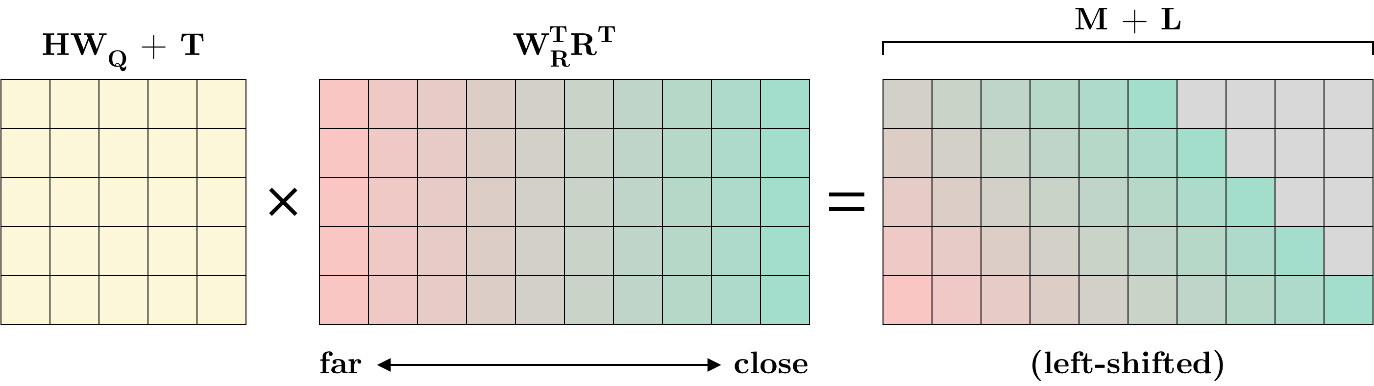
Figure 1: Combining $(b)$ and $(d)$ in a single matrix multiplication. Identical colors in the middle and right matrices do not represent equal values but only serve to more easily illustrate the idea of shifting.

For the first word in the current segment, the distance to the farthest word in memory is $M$ while for the last word it is $M+L-1$. To account for this, a “circulant” left-shift is applied to the rows of the matrix in $(b)$ and $(d)$. This ensures proper relative distances to previous words while the distance to subsequent words have their entries set to $0$⁶. This is illustrated in Figure 1 above. Also note that whereas positional encodings are only used prior to the first layer in a vanilla Transformer, Transformer-XL uses relative positional encodings in every layer.

Implementation

We have now covered the two primary innovations of Transformer-XL: The hidden state memory and the relative positional encodings required to make the memory work. Virtually all other parts of the model are identical to what you would find in a vanilla Transformer. We can thus proceed to an implementation of the model, starting with the multi-head attention mechanism, which constitutes the bulk of the code.

class MultiHeadAttention(nn.Module):
    def __init__(self, model_dim, embed_dim, mem_len, num_heads, dropout, R, device):
        super().__init__()
        
        self.R = R
        self.mem_len = mem_len
        self.embed_dim = embed_dim
        self.device = device
        
        self.u = nn.Parameter(torch.randn(1, num_heads, 1, embed_dim))
        self.t = nn.Parameter(torch.randn(1, num_heads, 1, embed_dim))
        
        self.w_q = nn.Linear(model_dim, num_heads*embed_dim, bias=False)
        self.w_k = nn.Linear(model_dim, num_heads*embed_dim, bias=False)
        self.w_v = nn.Linear(model_dim, num_heads*embed_dim, bias=False)
        self.w_r = nn.Linear(model_dim, num_heads*embed_dim, bias=False)
        
        self.dropout = nn.Dropout(dropout)
        self.mlp = nn.Linear(num_heads*embed_dim, model_dim, bias=False)
        self.layer_norm = nn.LayerNorm(model_dim)
    
    def forward(self, x, mem):
        # concat output from previous layer with "memory" from earlier segments
        h = torch.cat((mem, x), dim=1)
        
        batch_size, seg_len, _ = x.shape
        mem_len = h.shape[1] - seg_len
        total_len = h.shape[1]
        
        # compute projections of input and memory embeddings
        q = self.w_q(x).view(batch_size, seg_len, -1, self.embed_dim)
        k = self.w_k(h).view(batch_size, total_len, -1, self.embed_dim)
        v = self.w_v(h).view(batch_size, total_len, -1, self.embed_dim)
        r = self.w_r(self.R[-total_len:]).view(1, total_len, -1, self.embed_dim)
        
        # aligning matrices to (batch_size, num_heads, seg_len, embed_dim)
        q = q.transpose(1,2)
        k = k.transpose(1,2)
        v = v.transpose(1,2)
        r = r.transpose(1,2)
        
        # the "XL specific" way of computing the pre-softmax attention score
        ac = torch.einsum("bhid,bhjd->bhij", q + self.u, k)
        bd = torch.einsum("bhid,bhjd->bhij", q + self.t, r)
        bd = self.circulant_shift(bd, -seg_len+1)
        
        # computing the attention scores
        att_score = ac + bd
        att_score = att_score.tril(mem_len) / self.embed_dim**0.5
        att_score[att_score == 0] = float("-inf")
        att_score = torch.softmax(att_score, dim=-1)
        
        # compute output
        att = (att_score @ v).transpose(1,2).reshape(batch_size, seg_len, -1)
        out = self.dropout(self.mlp(att))
        return self.layer_norm(out + x)
              
    def circulant_shift(self, x, shift):
        """
        Shifts top row of `x` by `shift`, second row by `shift-1`, etc. This is
        used to compute the relative positional encoding matrix in linear time
        (as opposed to quadratic time for the naive solution). Note: Right-hand
        side values are not zeroed out here.
        
        See Appendix B of the Transformer-XL paper for more details.
        """
        batch_size, num_heads, height, width = x.shape
        i = torch.arange(width).roll(shift).unsqueeze(0).to(self.device)
        i = i.flip(1).repeat(1, 2)
        i = i.unfold(dimension=1, size=width, step=1).flip(-1).unsqueeze(0)
        i = i.repeat(batch_size, num_heads, 1, 1)[:, :, :height]
        return x.gather(3, i)

Most of what you see above you would also find in an implementation of the multi-head attention module of a regular Transformer. The first lines that differ are the definitions of self.u and self.t. These are the $\R^d$ vectors comprising the $U$ and $T$ matrices in $(2)$.

The most important lines above are the following:

ac = torch.einsum("bhid,bhjd->bhij", q + self.u, k)
bd = torch.einsum("bhid,bhjd->bhij", q + self.t, r)
bd = self.circulant_shift(bd, -seg_len+1)

Here, ac takes care of computing the sum of part $(a)$ and $(c)$ in $(2)$ using a single matrix multiplication. The sum of part $(b)$ and $(d)$ is computed similarly and stored in bd after which the resulting $\R^{L \times d}$ matrix is shifted using the circulant_shift method. This operation corresponds to the left-shift illustrated in the right-hand side of Figure 1. Note that we shift by -seg_len+1 or, equivalently, $L-1$. This ensures that each word has a distance of $0$ to itself, $1$ to its neighbor in memory, and so on. Since the attention score is masked in the forward method, there is no need to zero out entries in circulant_shift.

Most of the remaining code should be self-explanatory for anyone familiar with Transformers. The only thing left to cover is the implementation of the hidden states. We manage these in the TransformerXL class and, more specifically, in the following methods:

class TransformerXL(nn.Module):
    def forward(self, x):
        x = self.dropout(self.embed(x))
        
        # create memory tensors if they haven't been already
        if self.mem is None:
            batch_size = x.size(0)
            self.set_up_memory(batch_size)
        
        # compute model output, saving layer inputs to memory along the way
        for i, dec in enumerate(self.layers):
            x_ = x.clone()
            x = dec(x, self.mem[i])
            self.add_to_memory(x_, i)
            
        return self.out_layer(x)
        
    def set_up_memory(self, batch_size):
        self.mem = [torch.zeros(batch_size, 0, self.model_dim).to(self.device)
                    for _ in range(len(self.layers))]
    
    def add_to_memory(self, x, i):
        if self.mem_len == 0: return
        self.mem[i] = torch.cat((self.mem[i], x.detach()), dim=1)[:, -self.mem_len:]
    
    def clear_memory(self):
        self.mem = None

Here, dec refers to a decoder layer, which is a small wrapper around a multi-head attention layer followed by a position-wise feed-forward layer. As you can see, the inputs to each layer is continuously saved to memory, keeping only the $M$ (here represented by self.mem_len) most recent inputs.

Training the model

The code for training the model can be found in train.py on GitHub. We train the model to sort unordered sequences of $n$ digits from 0-9. For example, using sequences of length 4, the sequence [4,5,3,0] will be input to the model as [4,5,3,0,0,3,4]. This will produce 7 next-digit predictions of which we care about (and optimize with respect to) the last 4. Note that we use causal masking, such that each prediction cannot incorporate information about subsequent digits in the sequence. For a simple task like this, we can safely set $M=0$ during training.

Testing the model

Once the model has been trained using train.py, you can evaluate it using eval.py. In this case, we set $M=2n - 1$ (i.e. the sequence length and all predictions but the last) and start by inputting only the unordered sequence, e.g. [1,8,8,2]. The last prediction of this sequence will be the model’s prediction of the first digit in the sorted sequence, here 1 (hopefully). Now, instead of inputting [1,8,8,2,1], we simply input 1, since the representations of [1,8,8,2] have already been saved to memory and don’t need to be recomputed. We repeat this until the model has produced $n$ predictions. For good measure, we also evaluate the model with $M=0$ by continually inputting the whole unordered sequence along with the growing list of predicted digits. We then compare the performance with and without memory augmentation.

Evaluating without memory...
100%|██████████████████████████████████████████████████████████████████████████████| 5/5 [00:45<00:00,  9.03s/it]
Achieved accuracy of 0.9732000231742859 in 45.156030893325806 seconds

Evaluating with memory...
100%|██████████████████████████████████████████████████████████████████████████████| 5/5 [00:14<00:00,  2.97s/it]
Achieved accuracy of 0.9732000231742859 in 14.850011825561523 seconds

Evaluating the model locally on a CPU produces the output above and shows a performance increase of more than 3x when using the model’s memory. While significant, this improvement is, of course, far from the 1800x mentioned by the authors.

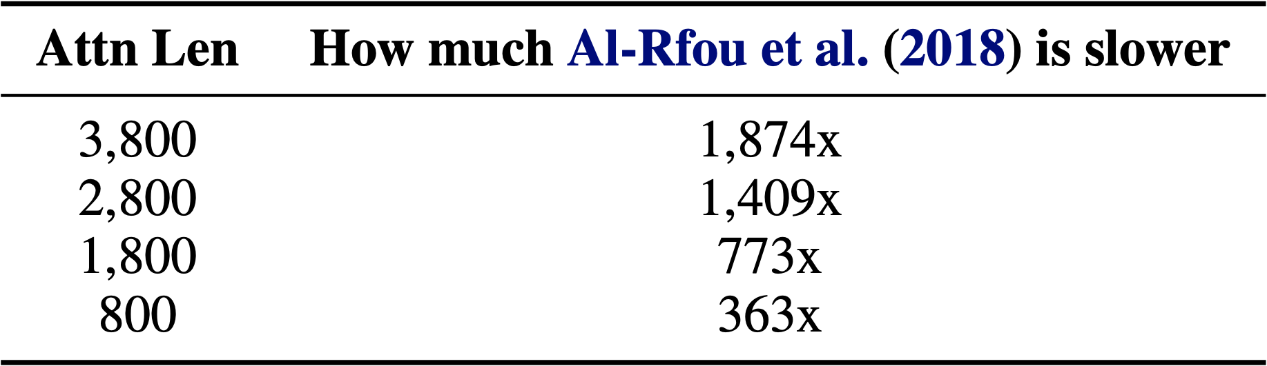
From Dai et al.¹

The reason for this is likely that the performance increase is highly dependent on the “attention length” (i.e. $M+L$), with smaller lengths resulting in less significant speedups. This is shown in the table above when compared to the work of Al-Rfou et al.⁷

Conclusion

The methods proposed in Transformer-XL are a simple but efficient way of widening the “receptive field” of a Transformer’s attention layers. If you would like to explore what the model is capable of when it is scaled up and trained on a large corpus of text, you can play around with the pretrained XLNet model available on HuggingFace. If you are more interested in exploring the nuts and bolts of the model architecture, I encourage you to check out the associated GitHub repo and give it a star if you find it helpful ⭐️

Notes and references