Self-Supervised Learning of Image Representations With VICReg

March 3, 2023

Code available on GitHub

How can we learn good image representations without the need for labeled datasets? Research in this area holds the promise of providing to the vision domain the same abundance of training data that has fueled progress in NLP. In this post, we will explore the problem of SSL through the lens of VICReg¹, a recent proposal for self-supervised learning of image representations proposed by researchers at Meta and published at ICLR 2022. We will implement our own version of the model and train it on CIFAR-10, making it feasible to run on a single GPU.

SSL in the vision domain

The most prominent use of SSL today is the training of LLMs. Here, a sequence of token embeddings is causally masked, and the model is trained to predict token $t$ given tokens $<t$. In vision, the closest analogue to this approach is to incorporate a temporal dimension (in the form of successive video frames) and training a model to predict frame $t$ given frames $<t$.

However, as Yann LeCun and Ishan Misra explain, such an approach is currently infeasible. This is due to the fact that the continuous and high-dimensional nature of images makes it much harder to represent uncertainty compared with the discrete and relatively low-dimensional nature of text, where a vocabulary can be easily vectorized and optimized using cross entropy.

Today, the most popular approaches to SSL in the vision domain instead rely on joint embedding architectures, where two different augmentations of the same image are input to separate branches of a model, each consisting of an encoder and a projector. Each branch outputs an embedding, and the model is trained to minimize the distance between pairs of embeddings corresponding to the same image. When the same architecture is used in both branches and share weights, this is known as a “siamese” architecture.

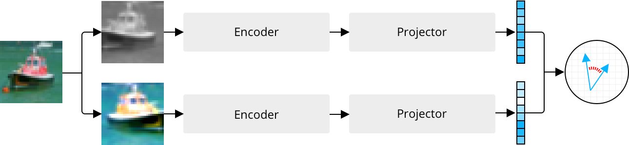
A joint embedding architecture is trained to produce similar embeddings for different augmentations of the same image.

The purpose of the encoder is to learn useful representations for downstream tasks such as image classification, while the projector is responsible for eliminating the information by which the two representations differ. Once the model has been trained, the projector is discarded², and the encoder can be fine-tuned for specific problems like image classification using much less labeled data than what is usually required when training in a purely supervised fashion.

Collapse

While this captures the basic idea behind self-supervised pre-training, it is not the whole story. If we blindly follow this approach, we will quickly discover that our models end up ignoring their inputs by collapsing their embeddings onto the zero-vector, thus minimizing the distance.

Broadly speaking, there are two approaches to combat the problem of collapse:

1. Contrastive approaches like SimCLR³ not only minimize the distance between embeddings corresponding to the same image (i.e. positive pairs), but also maximize the distance between embeddings corresponding to different images (i.e. negative pairs). By enforcing dissimilarity between negative pairs, collapsed embeddings become suboptimal.
2. Non-contrastive approaches dispense with negative pairs but currently do so in favor of poorly understood optimization tricks. For instance, BYOL⁴ uses a so-called momentum encoder, which anchors the parameters of one branch to an exponential moving average of the parameters of the other. More recently, SimSiam⁵ showed how the momentum encoder can be discarded by introducing an alternating stop-gradient operator for each branch.

Contrastive methods tend to require large numbers of negative pairs to learn meaningful representations. In the case of SimCLR, which relies on in-batch sampling of negative pairs, this has the unfortunate side-effect of increasing the batch size to thousands of images. Meanwhile, reliance on a momentum encoder means that a non-contrastive model like BYOL requires identical architectures in each branch. This makes the model unsuitable for multi-modal SSL tasks like those used in training CLIP⁶.

VICReg

Proposed by Bardes et al., VICReg (short for Variance-Invariance-Covariance Regularization) is a more recent approach to self-supervised pre-training using a joint embedding architecture. It alleviates many of the problems with previous methods, such as reliance on siamese networks, large batch sizes, and poorly understood optimization tricks. Instead, it proposes a simple and model-agnostic training procedure with an intuitive interpretation and performance on-par with other methods (75.5% Top-1 accuracy on ImageNet with a siamese ResNet-50 backbone).

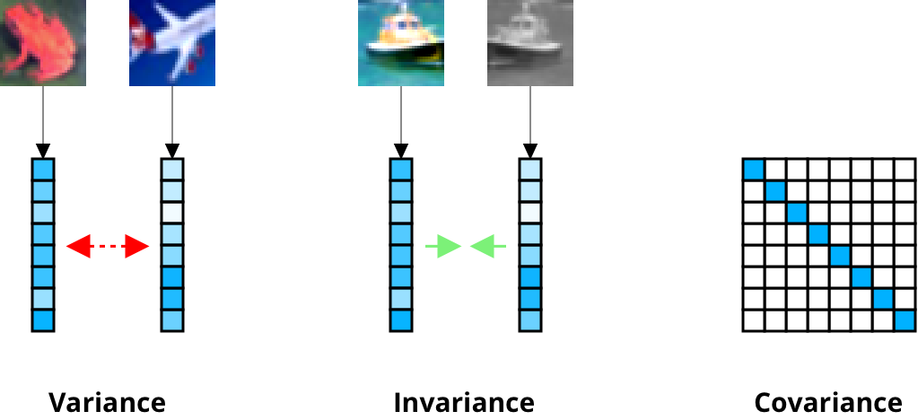
The novelty of VICReg lies in its loss function which consists of a variance term that repels negative pairs, an invariance term that attracts positive pairs, and a covariance term that prevents the individual components of each embedding from encoding similar information (think $\beta$-VAE⁷ and disentangled latent factors). Let’s go through each of these one by one.

The variance term $v(Z)$ below is defined for a batch $Z \in \mathbb{R}^{n \times d}$ of $n$ embeddings:

€€ v(Z) = \frac{1}{d} \sum_{j=1}^d \max(0, \gamma - \sqrt{\text{Var}(z^j) + \epsilon}), €€

Here, $z^j \in \mathbb{R}^n$ is the vector comprising the $j$’th element of all $n$ embeddings and $\gamma$ is a target standard deviation, which the authors set to $1$. Minimizing this expression drives the batch-wise standard deviation of each embedding dimension towards $\gamma$, thus encouraging diversity between negative pairs and preventing collapse.

Meanwhile, the invariance term below attracts positive pairs by minimizing the mean-squared Euclidean distance between embeddings $Z$ and $Z’$ of each branch:

€€ s(Z, Z’) = \frac{1}{n} \sum_{i=1}^n ||z_i - z_i’||^2_2 €€

The covariance term for a batch $Z$ is computed by first obtaining the covariance matrix $C(Z)$:

€€ C(Z) = \frac{1}{n-1} \sum_{i=1}^n (z_i - \mu)(z_i - \mu)^T, €€

where $\mu$ is the batch-wise mean vector. The covariance loss $c(Z)$ is then defined as

€€ c(Z) = \frac{1}{d} \sum_{i \neq j} [C(Z)]^2_{i,j}, €€

i.e. the average squared off-diagonal terms in the covariance matrix. Decorrelating the dimensions in this fashion prevents the embeddings from incorporating redundant information, thus maximizing their information content.

Loss coefficients

The variance term $v(Z)$, the invariance term $s(Z, Z’)$, and covariance term $c(Z)$ are gathered into the following loss function $\ell$, which is minimized during training:

€€ \ell(Z, Z’) = \lambda s(Z, Z’) + \mu [v(Z) + v(Z’)] + \nu [c(Z) + c(Z’)] €€

A proper configuration of the coefficients $\lambda$, $\mu$, and $\nu$ is required for the model not to collapse its representations onto the zero-vector. This is shown in the table below.

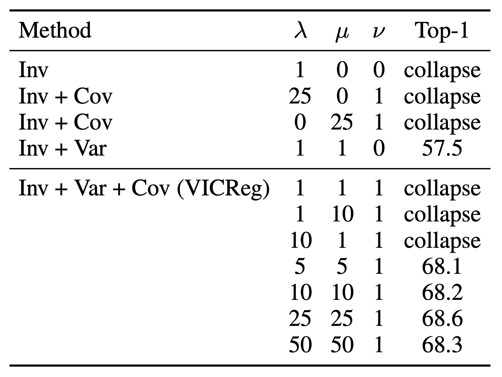
From appendix D.4 in the VICReg paper

The authors set $\lambda=25$, $\mu=25$, and $\nu=1$, which corresponds to the best result obtained in the table. They also mention that the same values work well on other datasets such as CIFAR-10. In our implementation, we will be using the same configuration.

It is interesting to note how much of a difference the covariance term makes in terms of downstream classification accuracy. By decorrelating the embedding dimensions, the accuracy shoots up from 57.5% to 68.6% Top-1 accuracy on ImageNet. If you are wondering why this accuracy is lower than the 75.5% mentioned above, this is due to the number of pre-training epochs used in the experiments. The results above were obtained after 100 epochs of pre-training while the 75.5% result was obtained after 1000 epochs.

Results on ImageNet

In the original paper, the authors use a ResNet-50 with output dimension 2048 as the encoder. Their projector is an MLP with two hidden layers of dimension 8192 as well as an output dimension of 8192. They evaluate the model on ImageNet and achieve the results below.

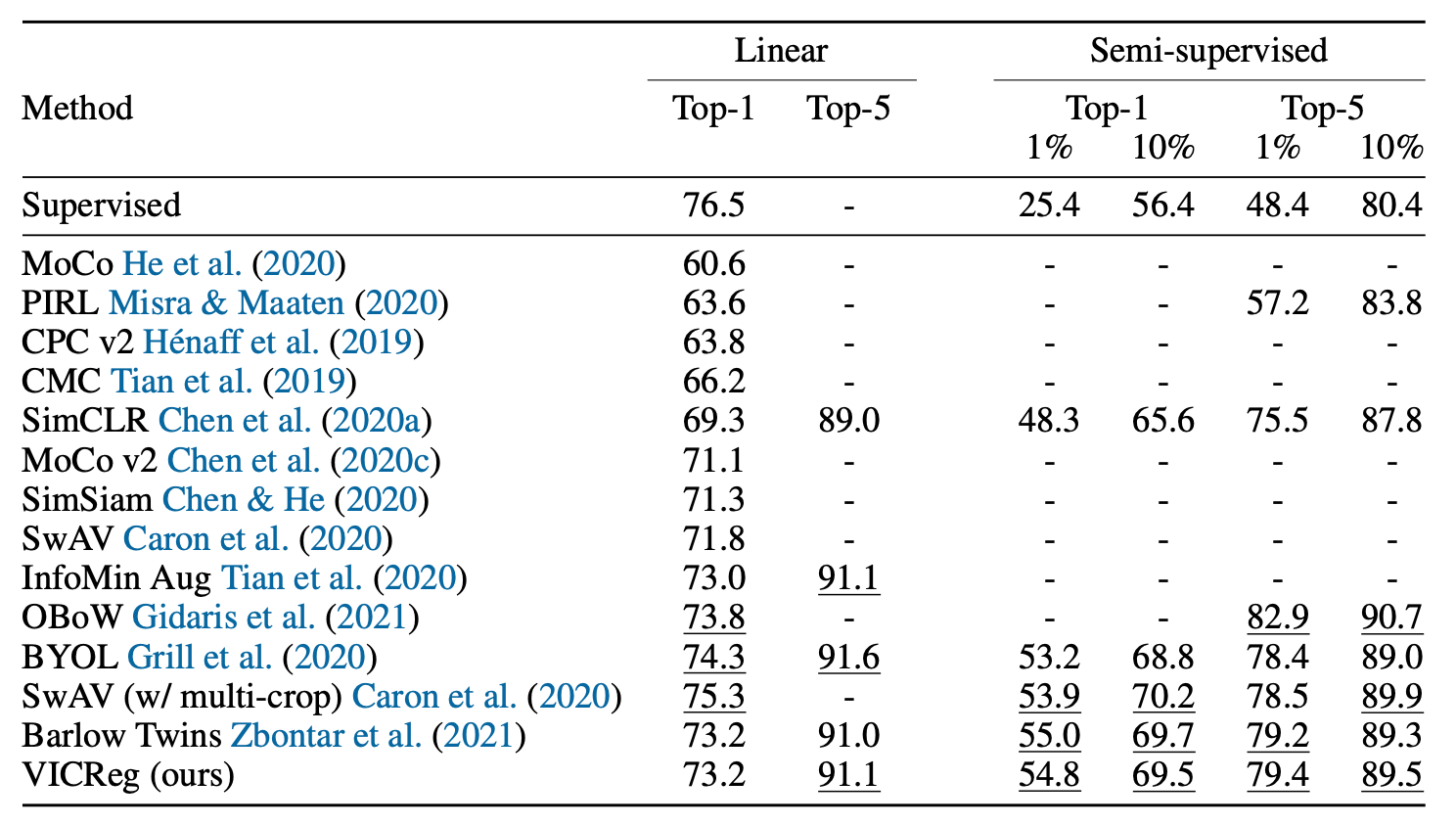
Here, “Linear” refers to the linear evaluation protocol, where a linear layer is added to the (frozen) encoder and trained for classification using the full training set. The resulting accuracy then acts as a proxy measure for representation quality. “Semi-supervised” refers to fine-tuning the linear layer and the encoder using only a subset (1% or 10%) of the training data.

Implementation

To keep things lightweight and feasible to run on a single GPU, we will implement the model using a ResNet-18 with output dimension 512. Our projector will be an MLP with two hidden layers and dimension 1024. We will evaluate it on CIFAR-10.

Let’s start by defining a simple Projector MLP using ReLU activations and batch normalization as prescribed in the paper:

class Projector(nn.Module):
    def __init__(self, encoder_dim, projector_dim):
        super().__init__()
        
        self.network = nn.Sequential(
            nn.Linear(encoder_dim, projector_dim),
            nn.BatchNorm1d(projector_dim),
            nn.ReLU(),
            nn.Linear(projector_dim, projector_dim),
            nn.BatchNorm1d(projector_dim),
            nn.ReLU(),
            nn.Linear(projector_dim, projector_dim),
            nn.BatchNorm1d(projector_dim),
            nn.ReLU(),
            nn.Linear(projector_dim, projector_dim)
        )
            
    def forward(self, x):
        return self.network(x)

We’ll then create a VICReg class wrapping a torchvision.models.resnet.resnet18 encoder and an instance of our Projector class.

class VICReg(nn.Module):
    def __init__(self, encoder_dim, projector_dim):
        super().__init__()
        
        self.encoder = resnet18(num_classes=encoder_dim)
        self.encoder.conv1 = nn.Conv2d(3, 64, kernel_size=(3,3), stride=1)
        self.encoder.maxpool = nn.Identity()
        
        self.projector = Projector(encoder_dim, projector_dim)
    
    def forward(self, x1, x2):
        x = torch.cat((x1, x2))
        y = self.encoder(x)
        return self.projector(y).chunk(2)

You’ll notice that we’re replacing the first convolutional layer of the ResNet encoder with a new Conv2d layer as well as replacing the max pooling layer with identity. This is because the ResNet architecture uses a $7 \times 7$ kernel in its first layer, since it is optimized for the much larger images in ImageNet. This is too reductive for the $32 \times 32$ images of CIFAR-10, so we’re replacing it with a $3 \times 3$ kernel and removing the max pooling. This is also the approach taken in the SimCLR paper when evaluating their model on CIFAR-10⁸.

We’ll then create the variance, invariance, and covariance functions

def variance(z, gamma=1):
    return relu(gamma - z.std(0)).mean()

def invariance(z1, z2):
    return mse_loss(z1, z2)

def covariance(z):
    n, d = z.shape
    mu = z.mean(0)
    cov = torch.einsum("ni,nj->ij", z-mu, z-mu) / (n - 1)
    off_diag = cov.pow(2).sum() - cov.pow(2).diag().sum()
    return off_diag / d

and next the randomized data augmentations used in training:

class Augmentation:
    augment = transforms.Compose([
        transforms.ToTensor(),
        transforms.RandomResizedCrop(size=32, scale=(0.2, 1.0)),
        transforms.RandomHorizontalFlip(0.5),
        transforms.RandomApply([transforms.ColorJitter(0.4, 0.4, 0.2, 0.1)], p=0.8),
        transforms.RandomGrayscale(0.2),
        transforms.RandomApply([transforms.GaussianBlur(3)], p=0.5),
        transforms.RandomSolarize(0.5, p=0.2),
        transforms.Normalize((0.4914, 0.4822, 0.4465), (0.247, 0.243, 0.261))
    ])
        
    def __call__(self, x):
        return self.augment(x), self.augment(x)

We’re wrapping the sequence of transformations in a class Augmentation, since this allows us to override __call__ and return two different augmentations for every input. By supplying an instance of Augmentation as the transform when specifying the dataset, our DataLoader will iterate over tuples of differently augmented batches, i.e.:

data = CIFAR10(root=".", train=True, download=True, transform=Augmentation())
dataloader = DataLoader(data, batch_size)

for images, labels in dataloader:
	x1 = images[0] # this is the batch augmented in one way
	x2 = images[1] # this is the same batch augmented in a different way

We can now train the model:

for epoch in tqdm(range(num_epochs)):
    for images, _ in dataloader:
        x1, x2 = images
        z1, z2 = model(x1, x2)
        
        la, mu, nu = 25, 25, 1
        var1, var2 = variance(z1), variance(z2)
        inv = invariance(z1, z2)
        cov1, cov2 = covariance(z1), covariance(z2)
        loss = la*inv + mu*(var1 + var2) + nu*(cov1 + cov2)
        
        opt.zero_grad()
        loss.backward()
        opt.step()

In the paper, the authors use the LARS optimizer⁹, which is tailored for training with large batch sizes. Since VICReg doesn’t require large batches, our implementation uses the more common Adam optimizer with learning rate $2 \cdot 10^{-4}$, default momentum parameters and a weight decay of $10^{-6}$. I encourage you to explore different optimizers and see how it affects performance (although this might be quite time-consuming depending on your hardware).

In my experience, the model keeps improving after 500 epochs of training with batch size 256, although slowly. At 500 epochs, the model achieves 85.5% accuracy on the CIFAR-10 test set in linear evaluation (see eval.py on GitHub). I suspect you can reach close to 90% if you let it train for at least another few hundred epochs. You can download the 500-epoch checkpoint here if you are interested in trying this.

Conclusion

The merits of self-supervised learning are obvious but the field is still figuring out how best to apply its methods outside of NLP. VICReg is but one such method, although an effective (and intuitive!) one. It’s interesting to consider the impact methods like this will have on computer vision in the not-so-distant future. Will computer vision, too, come to be dominated by large image models pre-trained on massive quantities of images and video, with everyone converging on a few “LIMs” for fine-tuning on downstream tasks like classification or segmentation? If so, we might have another “GPT moment” when pre-training is done not on the ~1M labeled images in ImageNet but 100 billion images scraped from the web.

Notes and references